 Leanpub
In this tutorial, we will be performing GNM calculations on one of the chains in the SARS-CoV-2 spike protein (6vxx) and then visualizing the results using the plots that we discussed in the main text.
We will be using ProDy, an open-source Python package that allows users to perform protein structural dynamics analysis. Its flexibility allows users to select specific parts or atoms of the structure for conducting normal mode analysis and structure comparison.
First, please install the following software:
We recommend creating a workspace for storing files when using ProDy or storing protein .pdb files. Open a terminal window and navigate to this workspace before starting IPython with the following command.
ipython --pylab
You will now need to import functions that we will use in this tutorial.
In[#]: from pylab import *
In[#]: from prody import *
In[#]: ion()
Finally, we turn on interactive mode (you only need to do this once per session).
In[#]: ion()
Next, we will parse in 6vxx.pdb and set it as the variable spike.
In[#]: spike = parsePDB('6vxx.pdb')
For this GNM calculation, we will focus only on the alpha carbons of Chain A. We can access these atoms using the spike.select function as follows, storing the alpha carbons in a variable calphas.
In[#]: calphas = spike.select('calpha and chain A')
Recall in the main text that we converted a protein into a network of nodes and springs, where two nodes are connected by an edge if the alpha carbons corresponding to these nodes are within some threshold distance \(r_c\). We can also represent this network with a matrix called the Kirchhoff matrix \(\Gamma\) and constructed as follows:
\[\Gamma_{ij} = \begin{cases} & -1 \text{ if $i \neq j$ and $R_{ij} \leq r_c$}\\ & 0 \text{ if $i \neq j$ and $R_{ij} > r_c$} \end{cases}\] \[\Gamma_{ii} = -\sum_j \Gamma_{ij}\]In other words, if residue i and j are connected to each other in the network, then the value of the (i, j)-th entry in the matrix will be -1. If these two residues are not connected, the the entry will be 0. The (i, j)-th entry on the main diagonal of \(\Gamma\), is equal to the total number of connections of residue i. The figure below shows an example Kirchhoff matrix for a small network.
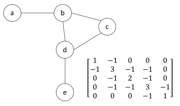 An example network (left) with its the corresponding Kirchhoff matrix (right).
The Kirchhoff matrix is helpful because applying some matrix algebra to it (specifically, determining its eigenvector decomposition) allows us to estimate the inner products \(\langle \Delta R_i, \Delta R_j \rangle\) that power the GNM model.
Returning to our SARS-CoV-2 example, we are now ready to build the Kirchhoff matrix. You can pass parameters for the cutoff (threshold distance between atoms) and gamma (spring constant). The defaults are 10.0 angstroms and 1.0, respectively. Here, we will set the cutoff to be 20.0 Å.
In[#]: gnm = GNM('SARS-CoV-2 Spike (6vxx) Chain A Cutoff = 20.0 A')
In[#]: gnm.buildKirchhoff(calphas, cutoff=20.0)
For normal mode analysis with ProDy, the default is 20 non-zero modes. In addition, we will create hinge sites for later use in the slow mode shape plot; these sites represent locations in the protein where fluctuations change in relative directions.
In[#]: gnm.calcModes()
In[#]: hinges = calcHinges(gnm)
For advanced users, information of the GNM and Kirchhoff matrix can be accessed with the following commands.
In[#]: gnm.getEigvals()
In[#]: gnm.getEigvecs()
In[#]: gnm.getCovariance()

#To get information specifically on the slowest mode (which is always indexed at 0):
In[#]: slowMode = gnm[0]
In[#]: slowMode.getEigval()
In[#]: slowMode.getEigvec()
We have now successfully initialized our GNM model and are ready to generate our plots. In what follows, make sure to save your visualization (if desired) and close each plot before creating another. We will discuss how to interpret these plots back in the main text.
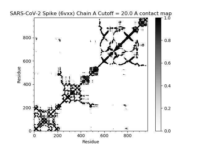
First, we produce a contact map, which we introduced earlier in the module.
In[#]: showContactMap(gnm);
This command should produce the following plot.
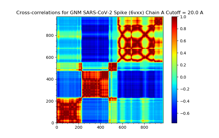
Next, we produce a cross-correlation plot with the following command.
In[#]: showCrossCorr(gnm);
The plot is found below.
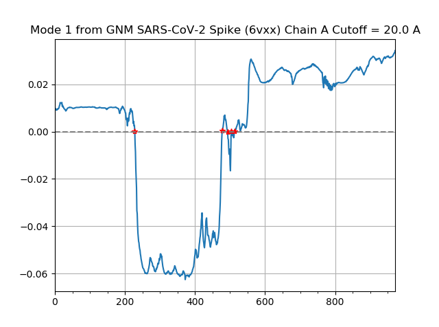
Finally, we use the following command to produce a shape plot for the slowest mode identified by GNM.
In[#]: showMode(gnm[0], hinges=True)
In[#]: grid();
This mode shape plot is shown in the figure below.
Now that we have produced our plots, we are ready to head back to the main text and analyze our results.
