 Leanpub
In this lesson, we will compare the results of the SARS-CoV-2 spike protein prediction from the previous lesson against each other and against the protein’s empirically validated structure. To do so, we need a method of comparing two structures.
Comparing two shapes with the Kabsch algorithm
Comparing two protein structures is intrinsically similar to comparing two shapes, such as those shown in the figure below.
STOP: Consider the two shapes in the figure below. How similar are they?
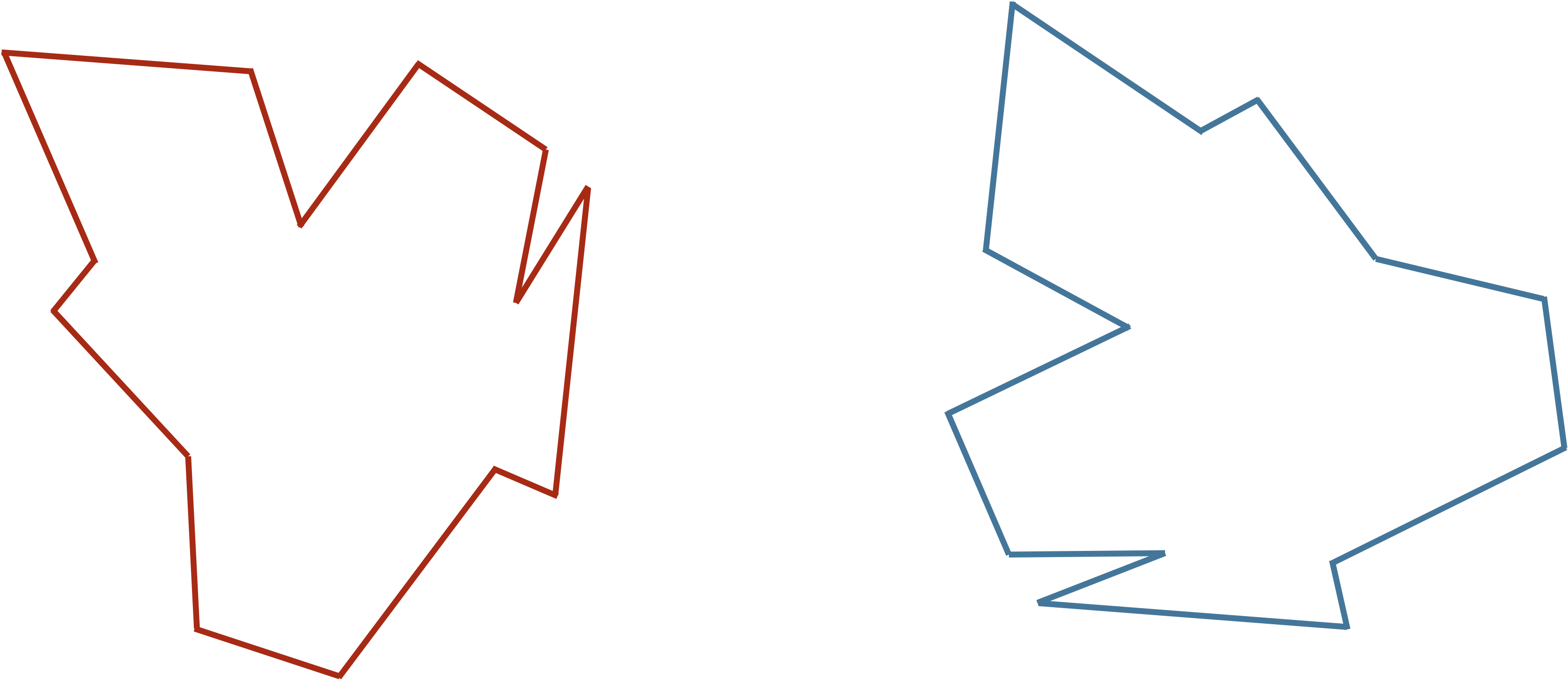
If you think you have a good handle on comparing the above two shapes, then it is because humans have very highly evolved eyes and brains. As we will see in the next module, training a computer to detect and differentiate objects is more difficult than you think!
We would like to develop a distance function d(S, T) quantifying how different two shapes S and T are. If S and T are the same, then d(S, T) should be equal to zero; the more different S and T become, the larger d should become.
You may have noticed that the two shapes in the preceding figure are, in fact, identical. To demonstrate that this is true, we can first move the red shape to superimpose it over the blue shape, then flip the red shape, and finally rotate it so that its boundary coincides with the blue shape, as shown in the animation below. In general, if a shape S can be translated, flipped, and/or rotated to produce shape T, then S and T are the same shape, and so d(S, T) should be equal to zero. The question is what d(S, T) should be if S and T are not the same shape.
 We can transform the red shape into the blue shape by translating it, flipping it, and then rotating it.
Our idea for defining d(S, T), then, is first to translate, flip, and rotate S so that it resembles T “as much as possible” to give us a fair comparison. Once we have done so, we should devise a metric to quantify the difference between the two shapes that will represent d(S, T).
We first translate S to have the same center of mass (or center of mass) as T. The center of mass of S is found at the point (xS, yS) such that xS and yS are the respective averages of the x-coordinates and y-coordinates on the boundary of S. The center of mass of some shapes can be determined mathematically. But for irregular shapes, we will first sample n points from the boundary of S and then estimate xS and yS as the average of all the respective x- and y-coordinates from the sampled points.
Next, imagine that we have found the desired rotation and flip of S that makes it resemble T as much as possible; we are now ready to define d(S, T) in the following way. We sample n points along the boundary of each shape, converting S and T into vectors s = (s1, …, sn) and t = (t1, …, tn), where si is the i-th point on the boundary of S. The root mean square deviation (RMSD) between the two vectors is the square root of the average squared distance between corresponding points,
\[\text{RMSD}(\mathbf{s}, \mathbf{t}) = \sqrt{\dfrac{1}{n} \cdot [d(s_1, t_1)^2 + d(s_2, t_2)^2 + \cdots + d(s_n, t_n)^2]} \,.\]In this formula, d(si, ti) is the distance between the points si and ti.
Note: RMSD is a common approach across data science when measuring the differences between two vectors.
For an example two-dimensional RMSD calculation, consider the figure below, which shows two shapes with four points sampled from each. (For simplicity, the shapes do not have the same center of mass.)
 Two shapes with four points sampled from each.
The distances between corresponding points in this figure are equal to \(\sqrt{2}\), 1, 4, and \(\sqrt{2}\). As a result, we compute the RMSD as
\[\begin{align*} \text{RMSD}(\mathbf{s}, \mathbf{t}) & = \sqrt{\dfrac{1}{4} \cdot (\sqrt{2}^2 + 1^2 + 2^2 + \sqrt{2}^2)} \\ & = \sqrt{\dfrac{1}{4} \cdot 9}\\ & = \sqrt{\dfrac{9}{4}}\\ & = \dfrac{3}{2} \end{align*}\]STOP: Do you see any issues with using RMSD to compare two shapes?
Even if we assume that two shapes have already been overlapped and rotated appropriately, we still should ensure that we sample enough points to give a good approximation of how different the shapes are. Consider a circle inscribed within a square, as shown in the figure below. If we happened to sample only the four points indicated in this figure, then we would sample the same points for each shape and conclude that the RMSD between these two shapes is equal to zero. Fortunately, this issue is easily resolved by making sure to sample enough points from the shape boundaries.
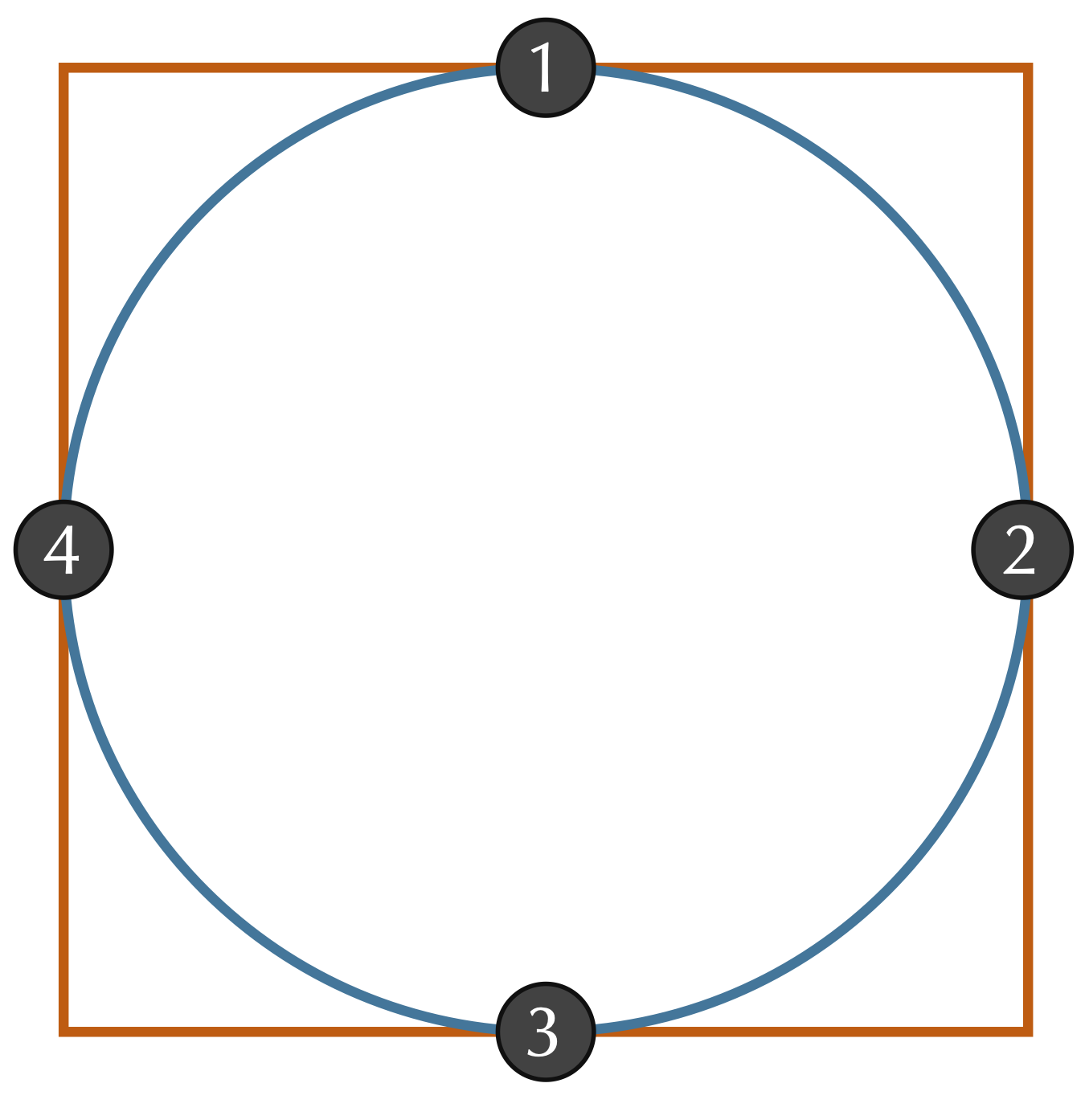 A circle inscribed within a square. Sampling of only the four points where the shapes intersect will give an RMSD of zero, a flawed estimate for the distance between the two shapes.
However, we have still assumed that we already rotated (and possibly flipped) S to be as “similar” to T as possible. In practice, after superimposing S and T to have the same center of mass, we would like to find the flip and/or rotation of S that minimizes the RMSD between our vectorizations of S and T over all possible ways of flipping and rotating S. It is this minimum RMSD that we define as d(S, T).
The best way of rotating and flipping S so as to minimize the RMSD between the resulting vectors s and t can be found with a method called the Kabsch algorithm. Explaining this algorithm requires some advanced linear algebra and is beyond the scope of our work but is described here.
PDB format represents a protein’s structure
The Kabsch algorithm offers a compelling way to determine the similarity of two protein structures. We can convert a protein containing n amino acids into a vector of length n by selecting a single representative point from each amino acid. For this representative point, we typically use the alpha carbon, the amino acid’s centrally located carbon atom.
Whether a protein structure is experimentally validated or predicted by an algorithm, the structure is often represented in a unified file format used by the PDB called .pdb format. In this format (see the figure below), each atom in the protein is labeled according to several different characteristics, including:
- the element from which the atom derives;
- the amino acid in which the atom is contained;
- the chain on which this amino acid is found;
- the position of the amino acid within this chain; and
- the 3D coordinates (x, y, z) of the atom in angstroms (10-10 meters).
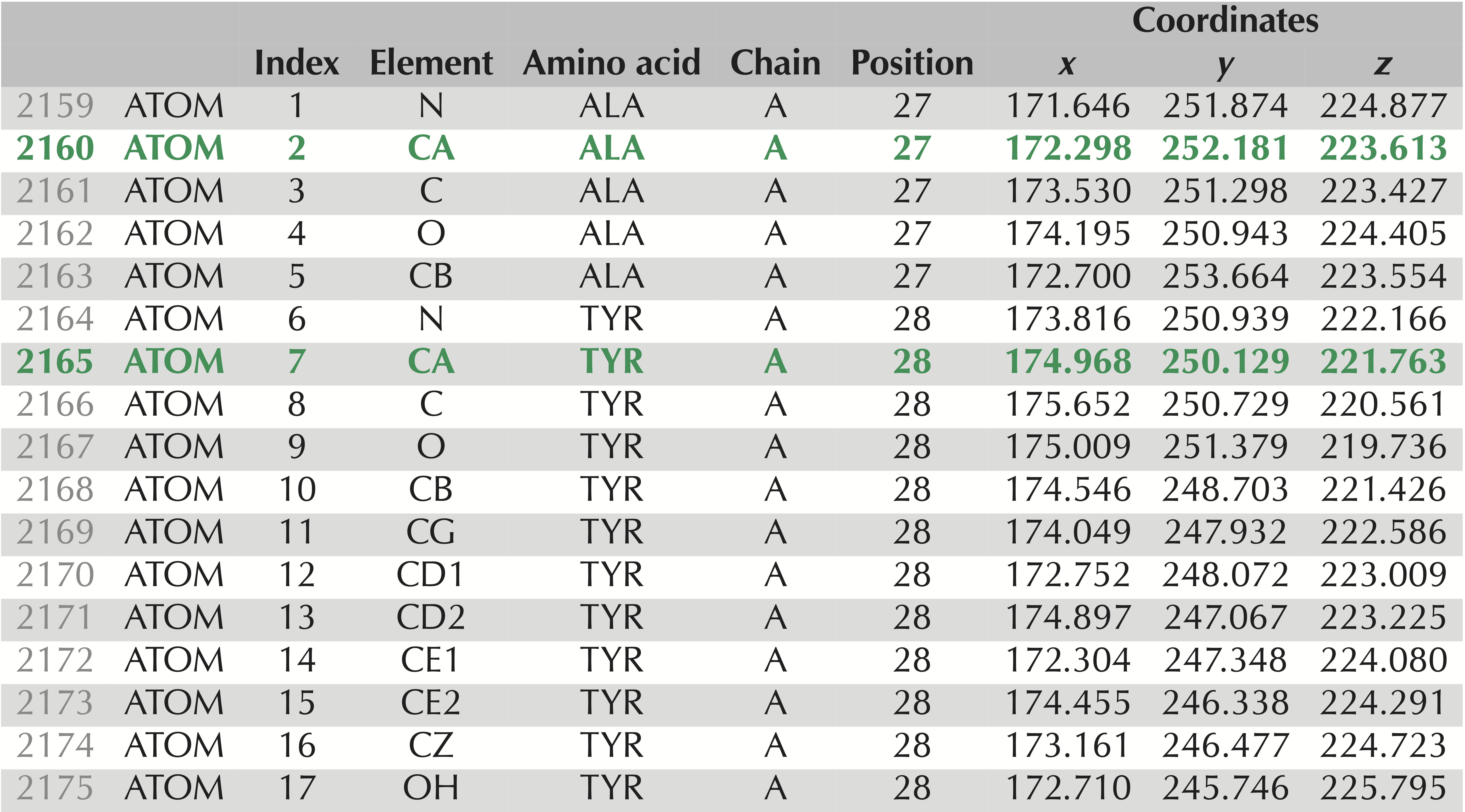 Lines 2,159 to 2,175 of the
 .pdb file for the experimentally verified SARS-CoV-2 spike protein structure, PDB entry 6vxx. These 17 lines contain information on the atoms taken from two amino acids, alanine and tyrosine. The rows corresponding to these amino acids’ alpha carbons are shown in green and appear as “CA” under the “Element” column. Column labels are as follows: “Index” refers to the number of the amino acid; “Element” identifies the chemical element to which this atom corresponds; “Chain” indicates which chain on which the atom is found; “Position” identifies the position in the protein of the amino acid from which the atom is taken; “Coordinates” indicates the x, y, and z coordinates of the atom’s position (in angstroms).
Note: The above figure shows just part of the information needed to fully represent a protein structure. For example, a .pdb file will also contain information about the disulfide bonds between amino acids. For more information, consult the official PDB documentation).
The Kabsch algorithm can be fooled
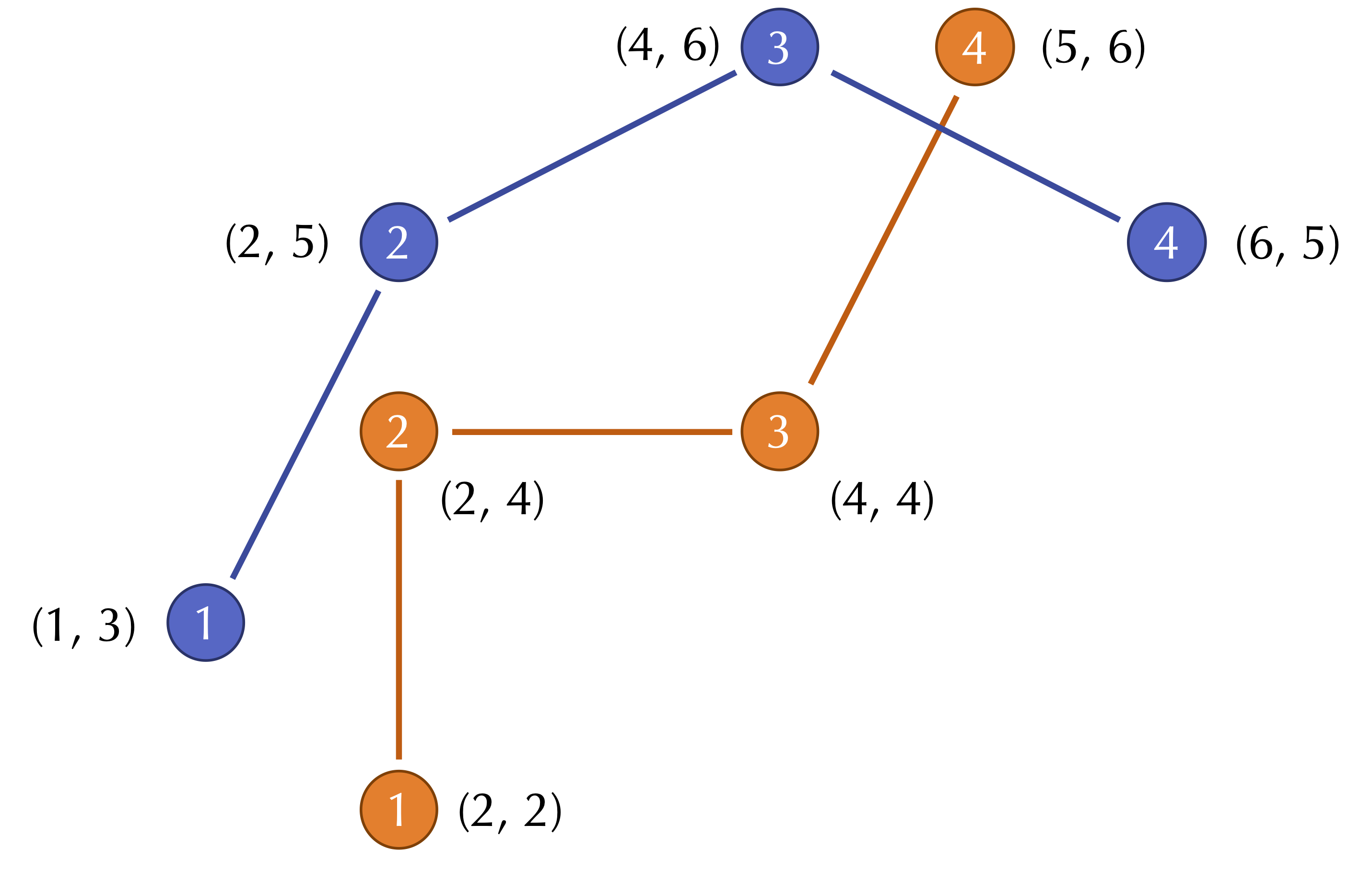
Although the Kabsch algorithm is powerful, we should be careful when applying it. Consider the figure below, which shows two toy protein structures; the orange structure (S) is identical to the blue structure (T) except for a change in a single bond angle between the third and fourth amino acids. And yet this tiny change in the protein’s structure causes a significant increase in d(si, ti) for every i greater than 3, which inflates the RMSD.
 (Top) Two hypothetical protein structures that differ in only a single bond angle between the third and fourth amino acids, shown in red. Each circle represents an alpha carbon. (Bottom left) Superimposing the first three amino acids shows how much the change in the bond angle throws off the computation of RMSD by increasing the distances between corresponding alpha carbons. (Bottom right) The Kabsch algorithm would align the centers of gravity of the two structures in order to minimize RMSD between corresponding alpha carbons. This alignment belies the similarity in the structures and makes it difficult for the untrained observer to notice the proteins’ similarity.
Another way in which the Kabsch algorithm can be tricked is in the case of an appended substructure that throws off the ordering of the amino acids. The following figure shows a toy example of a structure into which we incorporate a loop, thus throwing off the natural order of comparing amino acids. (The same effect is caused if one or more amino acids are deleted from one of the two proteins.)
 Two toy two protein structures, one of which includes a loop of three amino acids. After the loop, each amino acid in the orange structure will be compared against an amino acid that occurs farther long in the blue structure, thus increasing d(si, ti)2 for each such amino acid.
To address this second issue, biologists often first align the sequences of two proteins, discarding any amino acids that do not align before performing a vectorization of structures for the RMSD calculation. We will soon see an example of a protein sequence alignment when comparing the coronavirus spike proteins.
In short, if the RMSD of two proteins is large, then we should be wary of concluding that the proteins are very different, and we may need to combine RMSD with other methods of structure comparison. But if the RMSD is small (e.g., just a few angstroms), then we can have confidence that the proteins are indeed similar.
We are now ready to apply the Kabsch algorithm to compare the structures that we predicted for human hemoglobin subunit alpha and the SARS-CoV-2 spike protein against their respective experimentally validated structures.
Assessing the accuracy of our structure prediction models
In the tutorials occurring earlier in this module, we used protein structure prediction software to predict the structure of human hemoglobin subunit alpha (using ab initio modeling) and the SARS-CoV-2 spike protein (using homology modeling). We will now see how well our models performed by showing the values of RMSD produced by the Kabsch algorithm when comparing each of these models against the validated structures.
Ab initio (QUARK) models of Human Hemoglobin Subunit Alpha
The table below shows the RMSD between each of the five predicted structures returned by QUARK and the validated structure of human hemoglobin subunit alpha (PDB entry: 1si4). We are tempted to conclude that our ab initio prediction was a success. However, because human hemoglobin subunit alpha is so short (141 amino acids), researchers would consider this RMSD score to be high.
| Quark Model | RMSD |
|---|---|
| QUARK1 | 1.58 |
| QUARK2 | 2.0988 |
| QUARK3 | 3.11 |
| QUARK4 | 1.9343 |
| QUARK5 | 2.6495 |
It is tempting to conclude that our ab initio prediction was a success. However, because human hemoglobin subunit alpha is such a short protein (141 amino acids), researchers would consider this RMSD score high.
Homology models of the SARS-CoV-2 spike protein
In the homology tutorial, we used SWISS-MODEL and Robetta to predict the structure of the SARS-CoV-2 spike protein, and we used GalaxyWeb to predict the structure of this protein’s receptor binding domain (RBD).
GalaxyWEB
First, we consider the five GalaxyWEB models produced for the spike protein RBD. The following table shows the RMSD between each of these models and the validated SARS-CoV-2 RBD (PDB entry: 6lzg).
| GalaxyWEB | RMSD |
|---|---|
| Galaxy1 | 0.1775 |
| Galaxy2 | 0.1459 |
| Galaxy3 | 0.1526 |
| Galaxy4 | 0.1434 |
| Galaxy5 | 0.1202 |
All of these models have an excellent RMSD score and can be considered very accurate. Note that their RMSD is more than an order of magnitude lower than the RMSD computed for our ab initio model of hemoglobin subunit alpha, despite the fact that the RBD is longer (229 amino acids).
SWISS-MODEL
We now shift to homology models of the entire spike protein and start with SWISS-MODEL. The following table shows the RMSD between each of three structures produced by SWISS-MODEL and the validated structure of the SARS-CoV-2 spike protein (PDB entry: 6vxx).
| SWISS MODEL | RMSD |
|---|---|
| SWISS1 | 5.8518 |
| SWISS2 | 11.3432 |
| SWISS3 | 11.3432 |
The first structure has a lowest RMSD over the three models, and even though its RMSD (5.818) is significantly higher than what we saw for the GalaxyWEB prediction for the RBD, keep in mind that the spike protein is 1281 amino acids long, and so the sensitivity of RMSD to slight changes should give us confidence that our models are on the right track.
Robetta
Finally, we produced five predicted structures of a single chain of the SARS-CoV-2 spike protein using Robetta. The following table compares each of them against the validated structure of the SARS-CoV-2 spike protein (PDB: 6vxx).
| Robetta | RMSD |
|---|---|
| Robetta1 | 3.1189 |
| Robetta2 | 3.7568 |
| Robetta3 | 2.9972 |
| Robetta4 | 2.5852 |
| Robetta5 | 12.0975 |
STOP: Which do you think performed more accurately on our predictions: SWISS-MODEL or Robetta?
Distributing protein structure prediction around the world
While some researchers were working to elucidate the structure of the SARS-CoV-2 spike protein experimentally, thousands of users were devoting their computers to the cause of predicting the protein’s structure computationally. Two leading structure prediction projects, Rosetta@home and Folding@home, encourage volunteers to download their software and contribute to a gigantic distributed effort to predict protein shape. Even with a modest laptop, a user can donate some of their computer’s idle resources to help predict protein structure.
The results of the SSGCID models of the S protein released by Rosetta@Home are shown below.
| SSGCID | RMSD (Full Protein) | RMSD (Single Chain) |
|---|---|---|
| SSGCID1 | 3.505 | 2.7843 |
| SSGCID2 | 2.3274 | 2.107 |
| SSGCID3 | 2.12 | 1.866 |
| SSGCID4 | 2.0854 | 2.047 |
| SSGCID5 | 4.9636 | 4.6443 |
As we might expect due to having access to thousands of users’ computers, the SSGCID models outperform our SWISS-MODEL models. Yet a typical threshold for whether a predicted structure is accurate is if, when compared to a validated structure, its RMSD is smaller than 2.0 angstroms, a test that the models in the above table do not pass.
The inability of even powerful models to obtain an accurate predicted structure for the SARS-CoV-2 spike protein may make it seem that protein structure prediction is a lost cause. Perhaps biochemists should head back to their expensive experimental validations and ignore the musings of computational scientists. In the conclusion to part 1, we will find hope.
