 Leanpub
In a previous tutorial, we segmented and binarized a collection of WBC images. If you completed that tutorial, then you should see those images as a collection of .tiff files in your BWImgs_1 folder inside your WBC_PCAPipeline/Data directory.
We are now ready to use CellOrganizer to build a shape space of these images and then apply PCA to the resulting shape vectors in order to reduce the dimension of the dataset.
Note: Currently, this tutorial only works for Mac and Linux users. We have created an alternative version of this tutorial for Windows users, which uses CellOrganizer for Docker, available here.
Note: If you are not interested in following this tutorial, or you hit a snag, we are providing the final shape vectors post-PCA in the following file: WBC_PCA.csv. Once this file is downloaded, you can also skip down to shape space visualization.
Installing CellOrganizer
First, as in the previous tutorial, you will need the latest version of MATLAB. You should then download the latest version of CellOrganizer for MATLAB, which you can find under Downloads at the CellOrganizer homepage. After downloading a .zip file, extract this file into a folder, and then place this folder somewhere on your computer where you will remember it. (Our suggestion is to place the folder in the same applications folder where MATLAB is found.)
To install CellOrganizer, open MATLAB, and in the command window navigate to the CellOrganizer folder that you just extracted by using the cd command. For example, if you are using MacOS, and you extracted the CellOrganizer folder as cellorganizer-master and moved it to your Applications folder, then you would type the following command:
cd /Applications/cellorganizer-master
Once you have navigated into this folder, you will see the contents of your CellOrganizer directory appear under the Current Directory window in MATLAB, as shown below.
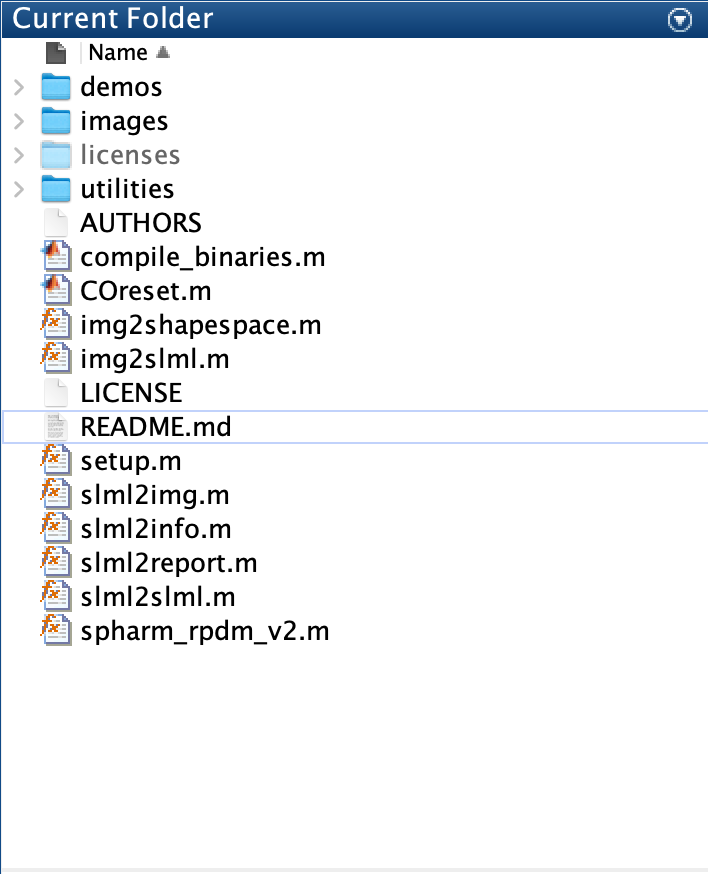
You are now ready to install CellOrganizer by running setup.m. To do so, enter the following command into the MATLAB command window.
setup();
That’s it! If your installation was successful, then you should see a message in the MATLAB command window similar to the following.
Adding appropiate folders to path.
Checking if your system and Matlab version is compatible with CellOrganizer.
Checking for updates. CellOrganizer version 2.9.2 is the latest stable release.
Keep MATLAB open, as we will be using it in the next step.
Generating a PCA Model
CellOrganizer has several different models to perform a collection of cell modeling tasks; we will focus on demo2D08, which will generate a PCA model for our white blood cell nucleus images. All of the necessary code for doing so is contained in WBC_PCAModel.m, a MATLAB file contained within the WBC_PCAPipeline/Step3_ModelGeneration directory. We will not walk through all the details of this file, but feel free to open this file with a text editor.
Run the following commands in the MATLAB command window to navigate into the WBC_PCAPipeline/Step3_ModelGeneration directory and then run WBC_PCAModel.m.
clear
clc
cd ~/Desktop/WBC_PCAPipeline/Step3_ModelGeneration
WBC_PCAModel
Note: These runs will generate a large amount of console output. You may want to go make a cup of coffee.
The run will be complete when you see output analogous to the following.
CLEAN UP WORKSPACE AND ENVIRONMENT
Removing temporary folder
Checking if model file exists on disk
Elapsed time is 11.682268 seconds.
Creating output directory /Users/phillipcompeau/Desktop/WBC_PCAPipeline/Step3_ModelGeneration/report
Number of objects: 345
As a result, the Step3_PCAModel and Step4_Visualization directories have been updated. The principal components along with the assigned label to each cell are captured in the WBC_PCA.csv file within the Step4 directory. Information about the images used and the shape space that CellOrganizer generated can be found in Step3_PCAModel/report/index.html.
Note: If you run the WBC_PCAModel.m file more than once, make sure to delete any log and param files that have been created from a previous run. All other files will be overwritten unless preemptively removed from the WBC_PCAModel file’s access. Saving the files can be done by either compressing the files into a zip folder or removing them from the directory.
Now that CellOrganizer has vectorized the images and applied PCA to the resulting shape vectors, we would like to explore the resulting vectors for each image. (Recall from the main text that these vectors are the original shape vectors projected onto the “nearest” hyperplane.)
First, run the following commands in the MATLAB command window:
load('WBC_PCA.mat');
scr = model.nuclearShapeModel.score;
Then, double-click on the scr variable in the Workspace window.
In the matrix on your screen, each row represents the coordinates for the projection of a single image’s shape vector.
An important point is that the first d columns in this matrix correspond to the vector’s projection onto the d-dimensional hyperplane minimizing the sum of squared distances from each shape vector to this hyperplane. For the purpose of our shape space visualization, we will only be focusing on the first three columns of this matrix. In this way, even though each shape vector lives in a high-dimensional space, we will obtain a three-dimensional representation of the data that represents the data faithfully.
Shape Space Visualization
Having generated a PCA model from our WBC images, we are now ready to visualize the resulting simplified three-dimensional shape space with each cell labeled according to its type. To do so, we will use Python 3, so make sure you have installed Python 3.
In WBC_PCAPipeline/Step4_Visualization of our provided folder, we provide two Python files (WBC_CellFamily.py and WBC_CellType.py) that we will use for plotting to visualize our shape space and label each image. The first file will label each image by cell family (granulocyte, lymphocyte, or monocyte); the second will use five labels, subdividing granulocytes into basophils, eosinophils, and neutrophils.
First, we will label each image in the shape space by cell family. Open a new terminal window (the “Terminal” app on MacOS, and the “Command Prompt” app on Windows) and run the following commands to navigate to “Step 4” of the Pipeline and run our cell family plotter.
cd ~/Desktop/WBC_PCAPipeline/Step4_Visualization
python WBC_CellFamily.py
You can click, drag, and rotate the resulting plot to see the clusters of cell classes by color (a legend can be found in the upper right corner). Furthermore, an image file of this visualization is saved within WBC_PCAPipeline/Step4_Visualization as WBC_ShapeSpace_CF.png.
Note: You may need to close the window containing the shape space in order to be able to run additional commands in your terminal window.
Next, we will classify images by cell type. In a terminal window, run the following commands to label the shape space according to each of the five cell types. An image of this visualization will be saved within WBC_PCAPipeline/Step4_Visualization as WBC_ShapeSpace_CT.png.
cd ~/Desktop/WBC_PCAPipeline/Step4_Visualization
python WBC_CellType.py
As we return to the main text, we will show the labeled shape space plots and return to the problem of classification.
