 Leanpub
Cross validation for WBC shape-space evaluation
We are nearly ready to apply k-NN to a dimension-reduced shape space of WBC nuclear images. However, we already know the correct class of every image in our dataset.
One approach for assessing the performance of a classification algorithm when the class of each object is known is to exclude some subset of the data, called the validation set. After hiding the correct classes for elements of the validation set from the classification algorithm, we will measure how often the algorithm correctly identifies the class of each object in the validation set.
STOP: What issues do you see with using a validation set?
Yet it remains unclear which subset of the data we should use as a validation set. Random variation could cause the classifier’s accuracy to change depending on which subset we choose. Ideally, we would use a more democratic approach that is not subject to random variation and that uses all of the data for validation.
In cross validation, we divide our data into a collection of f (approximately) equally sized groups called folds. We use one of these folds as a validation set, keeping track of which objects the classification algorithm classifies correctly, and then we start over with a different fold as our validation set. In this way, every element in our dataset will get used as a member of a validation set exactly once.
A first attempt at quantifying classifier performance on the iris dataset
Before we can apply cross validation to WBC images, we should discuss how to quantify the performance of the classifier. The table below shows the result of applying k-NN to the iris flower dataset, using k equal to 3 and cross validation with f equal to 10 (since there are 150 flowers, each fold contains 15 flowers). This table is called a confusion matrix, because it helps us visualize whether we are “confusing” the class assignment of an object.
In the confusion matrix, rows correspond to true classes, and columns correspond to predicted classes. For example, consider the second row, which corresponds to the flowers that we know are Iris versicolor. k-NN predicted that none of these flowers were Iris setosa, that 47 of these flowers were Iris versicolor, and that three of these flowers were Iris virginica. Therefore, it correctly predicted the class of 47 of the 50 total Iris versicolor flowers.
| Iris setosa | Iris versicolor | Iris virginica |
|---|---|---|
| 50 | 0 | 0 |
| 0 | 47 | 3 |
| 0 | 4 | 46 |
Note: We did not apply dimension reduction to the iris flower dataset because it has only four dimensions.
We define the accuracy of a classifier as the fraction of objects that it correctly identifies out of the total. For the above iris flower example, the confusion matrix indicates that k-NN has an accuracy of (50 + 47 + 46)/150 = 95.3%.
It may seem that accuracy is the only metric that we need. But if we were in a smarmy mood, then we might design a classifier that produces the following confusion matrix for our WBC dataset.
| Granulocyte | Monocyte | Lymphocyte |
|---|---|---|
| 291 | 0 | 0 |
| 21 | 0 | 0 |
| 33 | 0 | 0 |
STOP: What is the accuracy of this classifier?
Our clown classifier blindly assigned every image in the dataset to be a granulocyte, but its accuracy is 291/345 = 84.3%! To make matters worse, below is a confusion matrix for a hypothetical classifier on the same dataset that is clearly better but that has an accuracy of only (232 + 17 + 26)/345 = 79.7%.
| Granulocyte | Monocyte | Lymphocyte |
|---|---|---|
| 232 | 25 | 34 |
| 2 | 17 | 2 |
| 6 | 1 | 26 |
The failure of this classifier to attain the same accuracy as the one assigning the majority class to each element owes to the WBC dataset having imbalanced classes, which means that reporting only a classifier’s accuracy may be misleading.
For another example, say that we design a sham medical test for some condition that always comes back negative. If 1% of the population at a given point in time is positive for the condition, then we could report that our test is 99% accurate. But we would fail to get this test approved for widespread use because it never correctly identifies an individual who has the condition.
STOP: What other metrics could we design to measure a classifier’s success?
Recall, specificity, and precision
To motivate our discussion of other classifier metrics, we will continue with the analogy of medical tests, which can be thought of as classifiers with two classes (positive or negative).
First, we define some terms. A true positive is a positive test in a patient that has the condition; a false positive is a positive test in a patient that does not have the condition; a true negative is a negative test in a patient that does not have the condition; and a false negative is a negative test in a patient that does have the condition. The table below shows the locations of these four terms in the two-class confusion matrix for the test.
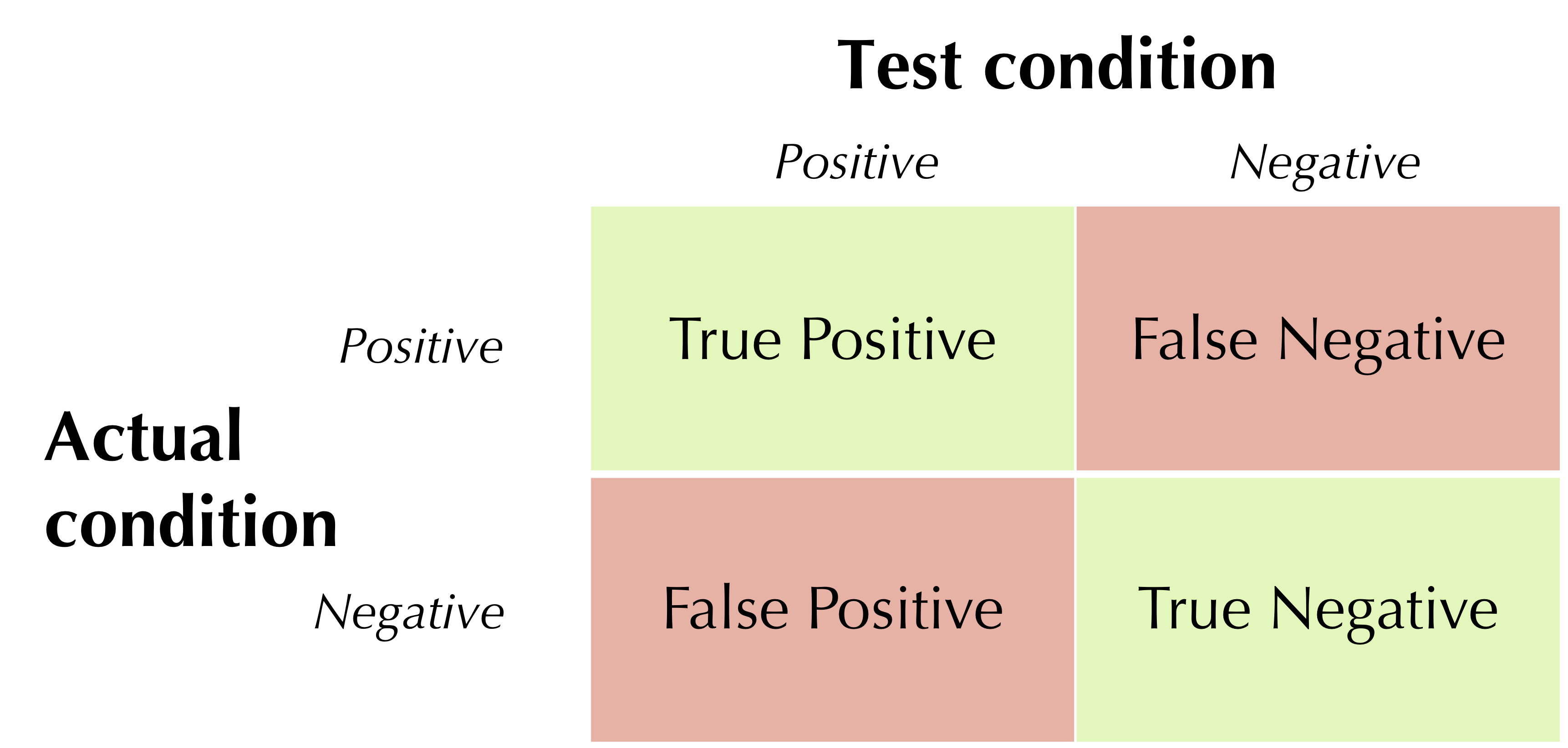 The locations of true positives, false positives, true negatives, and false negatives in the confusion matrix associated with a medical test. Correct predictions are shown in green, and incorrect predictions are shown in red.
In what follows, we will work with the confusion matrix for a hypothetical medical test shown in the figure below.
 A hypothetical medical test confusion matrix.
STOP: What is the accuracy of this test? How does it compare to the accuracy of a test that returns negative for everyone in the population?
Once again, this test has lower accuracy than one that returns negative for all individuals, but we will now show metrics for which it is superior.
The recall (a.k.a. sensitivity) of a two-class classifier is the percentage of positive cases that the test correctly identifies, or the ratio of true positives over the sum of the true positives and false negatives (found by summing the top row of the confusion matrix). For the confusion matrix in the table above, the recall is 1,000/(1,000 + 500) = 66.7%. Recall ranges from 0 to 1, with larger values indicating that the test is “sensitive”, meaning that it can identify true positives from a pool of patients who actually are positive.
The specificity of a test is an analogous metric for patients whose actual status is negative. Specificity measures the ratio of true negatives to the sum of true negatives and false positives (found by summing the second row of the confusion matrix). The hypothetical medical test has specificity equal to 198,000/(198,000 + 2,000) = 99%.
Finally, the precision of a test is the percentage of positive tests that are correct, or the ratio of true positives to the total number of positive tests (found by summing the first column of the confusion matrix). For example, the precision of our hypothetical medical test is 1,000/(1,000 + 2,000) = 33.3%.
STOP: How could we trick a test to have recall, specificity, or precision close to 1?
Just like accuracy, each of the above three of metrics is imperfect on its own and can be fooled by a frivolous test that always returns positive or negative. However, a frivolous test cannot score well on all these metrics at the same time. Therefore, in practice we will examine all these metrics, as well as accuracy, when assessing the quality of a classifier.
STOP: Consider a dataset of 201,500 patients, 1,500 of whom have a condition. Compute the recall, specificity, and precision of a medical test that always returns negative. How do these metrics compare against those of our hypothetical test?
You may find all these terms difficult to keep straight. You are not alone! An entire generation of scientists make copious trips to the Wikipedia page describing these and other classification metrics. After all, it’s called a confusion matrix for a reason…
Extending classification metrics to multiple classes
Before we return to our example of classifying images of WBC nuclei, we need to extend the ideas discussed in the preceding section to handle more than two classes. To do so, we consider each class individually and treat this class as the “positive” case and all other classes together as the “negative” case.
We use the iris flower dataset to show how this works. Say that we wish to compute the recall, specificity, and precision for Iris virginica using the k-NN confusion matrix that we generated, reproduced below.
| Iris setosa | Iris versicolor | Iris virginica |
|---|---|---|
| 50 | 0 | 0 |
| 0 | 47 | 3 |
| 0 | 4 | 46 |
We can simplify this confusion matrix into a two-class confusion matrix that combines the two classes corresponding to the other two species. The figure below shows this smaller confusion matrix, with Iris virginica moved to the first row and column.
| Iris virginica | Iris setosa and Iris versicolor |
|---|---|
| 46 | 4 |
| 3 | 97 |
This simplification allows us to compute classification statistics with respect to Iris virginica.
- recall: 46/(46+4) = 92%
- specificity: 97/(3+97) = 94%
- precision: 46/(46+3) = 93.9%
Once we have computed a statistic for each of the three iris species, we can then obtain a statistic for the classifier as a whole by taking the average of the statistics over all three species. For example, the overall recall of the classifier shown in the k-NN iris flower confusion matrix is the average of the recall for Iris setosa, Iris versicolor, and Iris virginica (which we just computed to be 92\%). We leave the computation of the other two recall values as an exercise.
STOP: Compute the recall, specificity, and precision for each of Iris setosa and Iris versicolor using the k-NN confusion matrix. Then, average each statistic over all three species to determine the classifier’s overall recall, specificity, and precision.
Let us consider one more example, returning to the confusion matrix for a hypothetical classifier on our WBC image dataset, reproduced below.
| Granulocyte | Monocyte | Lymphocyte |
|---|---|---|
| 232 | 25 | 34 |
| 2 | 17 | 2 |
| 6 | 1 | 26 |
The table below shows the computation of average recall, specificity, and precision for this classifier, which we previously mentioned has an accuracy of 79.7%.
| Count | Recall | Specificity | Precision | |
|---|---|---|---|---|
| Granulocyte | 291 | 79.725% | 85.185% | 96.667% |
| Monocyte | 21 | 80.952% | 91.975% | 39.535% |
| Lymphocyte | 33 | 78.788% | 88.462% | 41.935% |
| Average | 79.822% | 88.541% | 59.379% | |
| Weighted Average | 79.710% | 85.912% | 87.954% |
Note that the precision statistics for monocytes and lymphocytes weigh down the overall average precision of 59.379%. As a result, when we have imbalanced classes, we will also report the weighted average of the statistic, weighted over the number of elements in each class (see the final row in the above table). For example, the weighted average of the precision statistic is (291 · 96.667% + 21 · 39.535% + 33 · 41.935%)/(291 + 21 + 33) = 87.954%.
Now that we understand more about how to quantify the performance of a classifier, we are ready to apply k-NN to our WBC shape space (post-PCA of course!) and then assess its performance.
Applying a classifier to the WBC shape space
The confusion matrix shown below is the result of running k-NN on our WBC nuclear image shape space, using d (the number of dimensions in the PCA hyperplane) equal to 10, k (the number of nearest neighbors to consider when assigning a class) equal to 1, and f (the number of folds in cross validation) equal to 10.
| Granulocyte | Monocyte | Lymphocyte |
|---|---|---|
| 259 | 9 | 23 |
| 14 | 6 | 1 |
| 5 | 2 | 26 |
For these parameters, k-NN has an accuracy of 84.3% and a weighted average of recall, specificity, and precision of 84.3%, 69.4%, and 85.7%, respectively, as shown in the following table.
| Count | Recall | Specificity | Precision | |
|---|---|---|---|---|
| Granulocyte | 291 | 89.003% | 64.815% | 93.165% |
| Monocyte | 21 | 28.571% | 96.605% | 35.294% |
| Lymphocyte | 33 | 78.788% | 92.308% | 52.000% |
| Average | 65.454% | 84.576% | 60.153% | |
| Weighted Average | 84.348% | 69.380% | 85.705% |
If you explored the preceding tutorial, then you may wish to verify that these three values of d, k, and f appear to be close to optimal, in that changing them does not improve our classification metrics. We should ask why this is the case.
We start with d. If we set d too large, then once again the curse of dimension strikes. Using d equal to 344 (with k equal to 1 and f equal to 10) produces the baffling confusion matrix below, in which every element in the space is somehow closest to a lymphocyte.
| Granulocyte | Monocyte | Lymphocyte |
|---|---|---|
| 0 | 0 | 291 |
| 0 | 0 | 21 |
| 0 | 0 | 33 |
Using d = 3, we obtain better results, but we have reduced the dimension so much that we start to lose the signal in the data.
| Granulocyte | Monocyte | Lymphocyte |
|---|---|---|
| 257 | 15 | 19 |
| 16 | 5 | 0 |
| 20 | 0 | 13 |
We next consider k. It might seem that taking more neighbors into account would be helpful, but because of the class imbalance toward granulocytes, the effects of random noise mean that as we increase k, we will start considering granulocytes that just happen to be relatively nearby. For example, when k is equal to 5, every monocyte is classified as a granulocyte, as shown in the confusion matrix below (with d equal to 10 and f equal to 10).
| Granulocyte | Monocyte | Lymphocyte |
|---|---|---|
| 264 | 1 | 26 |
| 21 | 0 | 0 |
| 7 | 0 | 26 |
The question of the number of folds, f, is trickier. Increasing this parameter does not change the confusion matrix much, but in general, if we use too few folds (i.e., if f is too small), then we ignore too many known objects’ classes.
Yet we still have a problem. Although k-NN can identify granulocytes and lymphocytes quite well, it performs poorly on monocytes because of the class imbalance in our dataset. We have so few monocytes that encountering another one in the shape space simply does not happen often.
Statisticians have devised a variety of approaches to address class imbalance. We could undersample our data by excluding a random sample of the granulocytes. Undersampling works better when we have a large amount of data, so that throwing out some of the data does not cause problems. In our case, our dataset is small to begin with, and undersampling would risk plummeting the classifier’s performance on granulocytes.
We could also try using a different classification algorithm. One idea is to use a cost-sensitive classifier that charges a variable penalty for assigning an element to the wrong class, and then minimizes the total cost over all elements. For example, classifying a monocyte as a granulocyte would receive a greater penalty than classifying a granulocyte as a monocyte. A cost-sensitive classifier would help increase the number of images that are classified as monocytes, although it would also incorporate incorrectly classified monocyte.
Yet ultimately, k-NN outperforms much more advanced classifiers on this dataset. It may be a relatively simple approach, but k-NN offers a great match for classifying images within a WBC shape space, since proximity in this space indicates that two WBCs belong to the same family.
Limitations of our WBC image classification pipeline
Even though k-NN performed reasonably well on our WBC image dataset, we can still make improvements. After all, our model requires a number of steps from the intake of data to their ultimate classification, which means that several potential failure points could arise.
We will start with data. If we have great data, then a relatively simple approach will probably give a great result, but if we have bad data, then no amount of algorithmic wizardry will save us. An example of “good data” is the iris flower dataset; the features chosen were measured precisely and differentiate the flowers so clearly that it almost seems silly to run a classifier.
In our case, we have a small collection of very low resolution WBC images, which limits the performance of any classifier before we begin. Yet these data limitations are a feature of this chapter, not a bug, as they allow us to highlight a very common issue in data analysis. Now that we have built a classification pipeline, we should look for a larger dataset with higher-resolution images less class imbalance.
The next failure point in our model is our segmentation pipeline. Earlier in the module, we saw that this pipeline did not perfectly segment the nucleus from every image, sometimes capturing only a fragment of the nucleus. Perhaps we could exclude an image from downstream analysis if the segmented nucleus is below some threshold size.
We then handed off the segmented images to CellOrganizer to build a shape space from the vectorized boundaries of the nuclei. Even though CellOrganizer does what we tell it to do, the low resolution of the nuclear images will mean that the vectorization of each nuclear image is noisy.
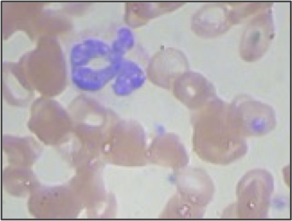
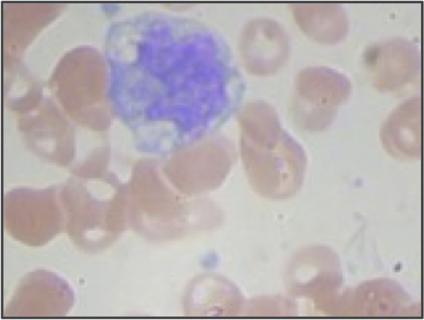
But even if we use higher resolution images and adjust our segmentation pipeline, we are still only building a model from the shape of the nucleus. We didn’t even take the size of the nucleus into account! If we return to the three sample WBC images from the introduction, reproduced in the figure below, then we can see that the lymphocyte nucleus is much smaller than the other two nuclei, which is true in general. When vectorizing the images, we could reserve an additional coordinate of each image’s vector for the size (in pixels) of the segmented nucleus. This change would hopefully help improve the performance of our classifier, especially on lymphocytes.

STOP: What other quantitative features could we extract from our images?
Finally, we discuss the classification algorithm itself. We used k-NN because it is intuitive to newcomers, but perhaps a more complicated algorithm could peer deeper into our dataset to find more subtle signals.
Ultimately, obtaining even moderate classification performance is impressive given the quality and size of our dataset, and the fact that we only modeled the shape of each cell’s nucleus. It also makes us wonder if we could improve this performance if we had access to a very high-quality dataset or a higher-powered computational approach. In this chapter’s conclusion, we discuss the foundations of an approach that not only constitutes the best known solution for WBC image classification but that is taking over the world.
