Shape Spaces

Stone tablets and lost cities

Imagine that you are a traveler to Earth and come across the ruins of New York City. You find an old road atlas that has a table of driving distances between cities (in miles), shown in the table below. Can you use this atlas to find the other cities in the table? In an earlier module, we encountered a “Lost Immortals” problem; this problem, of inferring the locations of cities given the distance between them, we call “Lost Cities”.

	New York	Los Angeles	Pittsburgh	Miami	Houston	Seattle
New York	0	2805	371	1283	1628	2852
Los Angeles	2805	0	2427	2733	1547	1135
Pittsburgh	371	2427	0	1181	1388	2502
Miami	1283	2733	1181	0	1189	3300
Houston	1628	1547	1388	1189	0	2340
Seattle	2852	1135	2502	3300	2340	0

STOP: If you know the locations of New York and Seattle, how could you use the information in the table above to find the other cities?

This seemingly contrived example has a real archaeological counterpart. In 2019, researchers used commercial records that had been engraved by Assyrian merchants onto 19th Century BCE stone tablets in order to estimate distances between pairs of lost Bronze age cities in present-day Turkey. Using this “atlas” of sorts, they estimated the locations of the lost cities.¹

You may be confused as to why biologists should care about stone tablets and lost cities. For now, we will return to our problem of classifying segmented WBC images by family.

Vectorizing a segmented image

As we mentioned in the previous lesson, we would like to apply k-NN to our example of segmented WBC images. Yet k-NN first requires each object to be represented by a feature vector, and so we need some way of converting a WBC image into a feature vector. In this way, we can produce a shape space, or an assignment of (cellular image) shapes to points in multi-dimensional space.

You may notice that the problem of “vectorizing” a WBC image is similar to one that we have already encountered in our module on protein structures. In that module, we vectorized a protein structure S as the collection of locations of its n alpha carbons to produce a vector s = (s₁, …, s_n), where s_i is the position of the i-th alpha carbon of S.

We will apply the same idea to vectorize our segmented WBCs. Given a binarized WBC nucleus image, we will first center the image so that its center of mass is at the origin, and then sample n points from the boundary of the cell nucleus to produce a shape vector s = (s₁, …, s_n), where s_i is a point with coordinates (x(i), y(i)).

Note: Both isolating the boundary of a binarized image and sampling points from this boundary to ensure that points are similarly spaced are challenging tasks that are outside the scope of our work here, and which we will let CellOrganizer handle for us.

To determine the “distance” between two images’ shape vectors, we will use our old friend root mean square deviation (RMSD), which is very similar to the Euclidean distance. Recall that the RMSD between shape vectors s and t is

\[\text{RMSD}(\mathbf{s}, \mathbf{t}) = \sqrt{\dfrac{1}{n} \cdot [d(s_1, t_1)^2 + d(s_2, t_2)^2 + \cdots + d(s_n, t_n)^2]}\,.\]

Inferring a shape space from pairwise distances

It is tempting to take the vectorization of every shape as our desired shape space. If this were the case, then we would hope that images of similarly shaped nuclei would have low RMSD and that the more dissimilar two nuclei become, the higher the RMSD of their shape vectors. The potential issues with this assumption are the same as those encountered when discussing protein structures, which we now review.

On the one hand, we need to ensure that the number of points that we sample from the object boundary is sufficiently high to avoid dissimilar shapes from having low RMSD. For this reason, CellOrganizer samples n = 1000 points by default for cell nuclei.

On the other hand, we could have very similar shapes whose RMSD winds up being high. For example, recall the shapes in the figure below, which are identical, but one has been flipped and rotated. If we were to vectorize these shapes as they are now in the same way (say, by starting at the top of the shape and proceeding clockwise), then we would obtain two vectors with high RMSD.

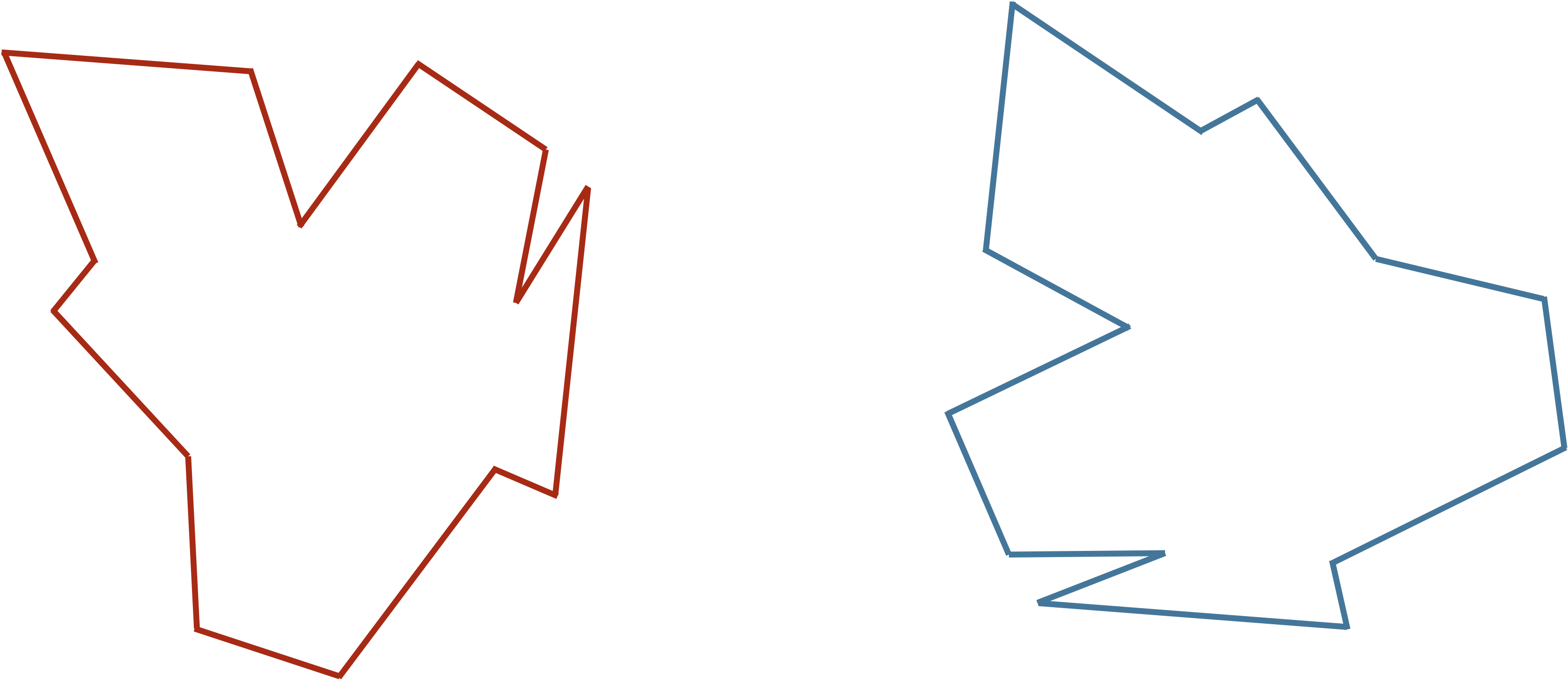Two identical shapes, with one shape flipped and rotated. Vectorizing these shapes without first correctly aligning them will produce two vectors with high RMSD.

We handled the latter issue in our work on protein structure comparison by introducing the Kabsch algorithm, which identified the best rotation of one shape into another that would minimize the RMSD of the resulting vectors. Yet what makes our work here more complicated is that we are not comparing two WBC image shape vectors, we are comparing hundreds.

We could apply the Kabsch algorithm to every pair of images, producing the RMSD between every pair of images. We would then need to build a shape space from all these distances between pairs of shapes. We hope that this problem sounds familiar, as it is the Lost Cities problem in disguise. The pairs of distances between images correspond to a road atlas, and placing images into a shape space corresponds to locating cities.

Note: CellOrganizer includes one model that applies an alternative approach to the Kabsch algorithm for computing a cellular distance, called the diffeomorphic distance², which can be thought of intuitively as determining the amount of energy required to deform one shape into another.

Statisticians have devised a collection of approaches called multi-dimensional scaling to solve versions of the Lost Cities problem that arise frequently in practice. The fundamental idea of multi-dimensional scaling is to assign points to n-dimensional space such that the distances between points in this space approximately resemble a collection of distances between pairs of objects in some dataset.

STOP: If we have m cellular images, then how many times will we need to compute the distance between a pair of images?

Aligning many images concurrently

Unfortunately, for a large image dataset, computing the distance between every pair of images can prove time-intensive, even with a powerful computer. Instead, we will rotate all images concurrently. After this alignment, we can then center and vectorize all the images starting at the same position.

One way of aligning a collection of images is to first identify the major axis of each image, which is the longest line segment that connects two points on the outside of the image and crosses through the image’s center of mass. The figure below shows the major axis for a few similar shapes.

Three similar shapes, with their major axes highlighted in gray.

Aligning the major axes of these similar shapes reveals their similarities (see figure below). These images are ready to be vectorized (say, starting from the point on the right side of an image’s major axis and proceeding counterclockwise). The resulting vectors will have low RMSD because corresponding points on the shapes will be nearby.

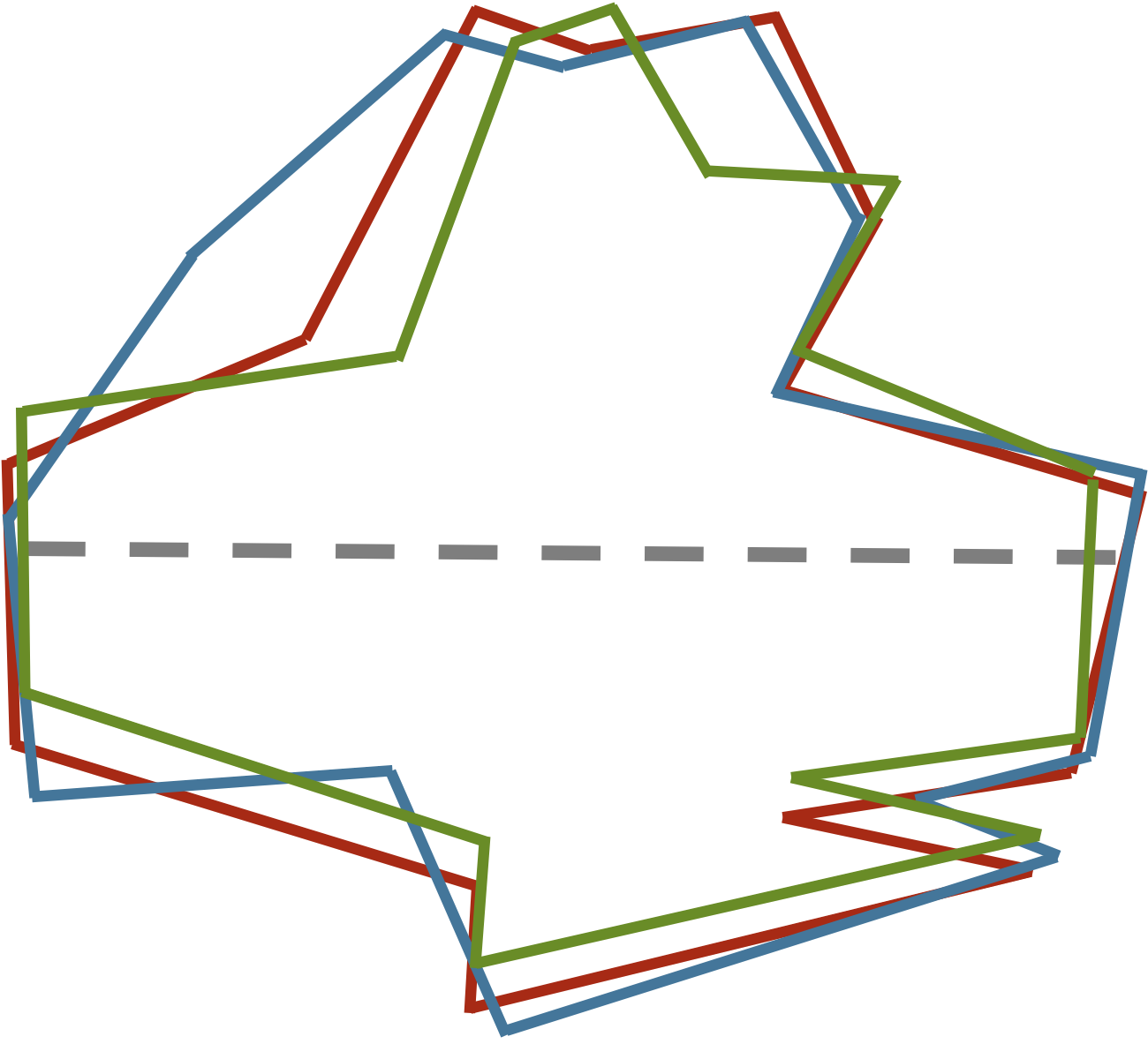Aligning the three images from the previous figure so that their major axes overlap allows us to see similarities between the shapes as well as build shape vectors for them having a consistent frame of reference.

Note: In practice, when we align shapes along their major axes, we need to consider the flip of each shape across its major axis as well. Handling this issue is beyond the scope of our work here but is discussed in the literature.³

By aligning and then vectorizing a collection of binarized cellular images after alignment, the resulting feature vectors form our desired shape space. We are almost ready to apply a classifier to this shape space, but one more pitfall remains.

Next lesson

1. Barjamovic B, Chaney T, Coşar K, Hortaçsu A (2019) Trade, Merchants, and the Lost Cities of the Bronze Age. The Quarterly Journal of Economics 134(3):1455-1503.Available online ↩

2. Rohde G, Ribeiro A, Dahl K, Murphy F (2008) Deformation-based nuclear morphometry: capturing nuclear shape variation in hela cells. Cytometry Part A 73:341–350.Available online ↩

3. Pincus Z, Theriot J (2007) Comparison of quantitative methods for cell-shape analysis. Journal of Microscopy 227(Pt 2):140-56.Available online ↩