 Leanpub
Installing R and RStudio
To run our segmentation pipeline, we will use R, a free programming language that is popular among data scientists across disciplines. We will also use RStudio, an integrated development environment that makes working with R easy.
You can download R and RStudio from their respective home sites or follow the instructions at Hands-On Programming with R.
Obtaining the WBC Image Data
The raw images and files that we will need to run our analysis are contained in a WBC_PCAPipeline folder that can be downloaded here as a .zip. Extract this file, move the resulting folder onto your desktop, and verify that it has the following contents:
WBC_PCAPipeline
	Data
		RawImgs
			BloodImage_00001.jpg
			·
			·
			·
			BloodImage_00410.jpg
		WBC_Labels.csv
	Step1_Segmentation
		WBC_imgSeg.R
	Step2_Binarization
		WBC_imgBin.m
	Step3_PCAModel
		WBC_PCAModel.m
	Step4_ShapeSpaceVisualization
		WBC_SS_CellClass.py
		WBC_SS_CellType.py
	Step5_Classification
	README.pdf
Note: Asking you to place this directory of files onto your desktop is unconventional. If you place it elsewhere, then you will have to manually change all file paths in the tutorials that follow in order to point to the appropriate directory. However, we have noticed occasional software glitches with using setwd() or pwd() if not specifying a universal location.
You may like to take a look at the Data folder, which contains the WBC images that we will work with in RawImgs. The other folders contain files that we will use to run different aspects of our analysis, starting with segmentation of the nuclei from the WBC images.
Segmenting Nuclei from WBC Images
In the main text, we stated that we would segment the nuclei from our WBC images by binarizing the image based on color. The nucleus shows up as bluish, so that our idea is to color a pixel white if it has above a certain threshold level of blue, below a threshold amount of red, and below a threshold amount of green.
Open RStudio, navigate to File --> Open File, and find Desktop/WBC_PCAPipeline/Step1_Segmentation/WBC_imgSeg.R. You should see the WBC_imgSeg.R file appear on the left side of the RStudio window.
The first few lines of WBC_imgSeg.R refer to a collection of three packages (or libraries) that we need to install in order to run segmentation pipeline. Two of these packages (jpeg and tiff) are contained in R, and the third (EBImage) is installed from the Bioconductor project as part of the BiocManager package. These package installations correspond to the following lines of our R file.
install.packages("jpeg")
install.packages("tiff")
install.packages("BiocManager")
BiocManager::install("EBImage")
Place your cursor on the first line of the file, and click Run, which will install the jpeg package along with any packages upon which it depends.
You can then click Run three more times to install each of the other three packages.
Note: Should you be asked in the RStudio console about upgrading dependencies during the EBImage library installation, type a and hit enter. Also, after you run this file once, should you decide to run this file again, you will not need to run the package installations and can comment them out using #.
Now that we have installed the required packages, we indicate to R that we want to use each of the three packages that we just installed in this file. Run each of the following three lines.
# Required Libraries
library("EBImage")
library("jpeg")
library("tiff")
Next, we run the following lines, which will create a directory counter that will keep track of how many files we have processed thus far.
# dir Counter
i = 1
We will now run commands to set paths for raw images and segmented images. segImgs will contain all of the segmented nuclei images in which the WBC nucleus is white and the rest of the image is in black. colImgs will contain all of the segmented nucleus images in which the nucleus retains its original color (and the background of the image is black). Finally, BWImgs will store binarized versions of our segmented images (more on this later).
# Set path for raw image files
path="~/Desktop/WBC_PCAPipeline/Data/"
rawImgs=paste(path, "RawImgs/", sep="")

# Set up directory path for segemented images
segImgs=paste(path, "SegImgs_", sep="")
colImgs=paste(path, "ColNuc_", sep="")
bwImgs=paste(path, "BWImgs_", sep="")
Next, we run commands to set up directories and print some messages to the console regarding the creation of these directories.
# Check if unique seg directory exists, otherwise create one
while (file.exists(paste(segImgs, toString(i), sep=""))) {
  i = i + 1
}
print(noquote(paste("Creating", paste(segImgs, toString(i), sep=""), "directory for segmented images.")))
dir.create(paste(segImgs, toString(i), sep=""), showWarnings = FALSE);
print(noquote(paste("Creating", paste(bwImgs, toString(i), sep=""), "directory for binarized images.")))
dir.create(paste(bwImgs, toString(i), sep=""), showWarnings = FALSE)
print(noquote(paste("Creating", paste(colImgs, toString(i), sep=""), "directory for nucleus in color images.")))
dir.create(paste(colImgs, toString(i), sep=""), showWarnings = FALSE)

outDir=paste(segImgs, toString(i), sep="")
setwd(rawImgs)

# Gather all files within the directory above
all.files <- list.files()
my.files <- grep("*.jpg", all.files, value=T)

print(noquote("Starting nucleus segmentation..."))
Finally, the engine of our work is a function that processes and segmentes every image individually according to the thresholding that we discussed above. Note that in the following code, a pixel is only retained if its red value is less than 65%, its green value is less than 60%, and its blue value is above 59.75% (see the values of r_threshold, g_threshold, and b_threshold).
We should only need to run the first line of the following code, since R will automatically perform everything inside this “for loop” for as many files as are in our dataset. You should not feel obligated to consult the following lines unless you are interested. The only thing that this code does that we have not discussed is that after segmentation, it identifies contiguous objects in the image and removes any objects whose area is smaller than some threshold, which allows us to remove any small artifacts from the image.
# Loop through each file and process each image individually
for (i in my.files) {
  print(noquote(paste("Segmenting nucleus from file", i)))
  # Read the image, change to its directory
  nuc = readImage(paste(rawImgs, i, sep=""))

  # Each nuclear stain has low red, low green and high blue.

  # Need to invert the red and green channels, and then threshold according to
  # the above criteria
  nuc_r = channel(nuc, 'r')
  nuc_g = channel(nuc, 'g')
  nuc_b = channel(nuc, 'b')

  # Assigned thresholds for low red, low green, and high blue.
  r_threshold = 0.65
  g_threshold = 0.60
  b_threshold = 0.5975

  # Apply the thresholds accordingly
  nuc_rTH = nuc_r < r_threshold
  nuc_gTH = nuc_g < g_threshold
  nuc_bTH = nuc_b > b_threshold

  nucleusComp = nuc_rTH & nuc_gTH & nuc_bTH
  nucleusBW = bwlabel(fillHull(nucleusComp))


  # Compute features for objects that have made the threshold boundaries
  features = computeFeatures.shape(nucleusBW)

  # Assigned area threshold
  area_threshold <- 1500

  # Find all features that do not meet the area threshold
  indices = which(features < area_threshold)
  nucleusFin = rmObjects(nucleusBW, indices)

  newFeatures = computeFeatures.shape(nucleusFin)

  # Write final nucleus image to disk
  filename = paste(outDir, i, sep="/")
  writeImage(nucleusFin, filename)
}
Finally, we print that we are finished. If we see this command printed to the console, then we know that we are finished.
print(noquote("DONE!"))
Note: If you run the file multiple times, three directories are created each time within the Data folder with the form of SegImgs_i, ColNuc_i, and BWImgs_i, where i is an integer. The images are only segmented into the most recently created directories (those with the largest value of i). Should you run into trouble and need to run this file multiple times, ensure that future file paths are pointing to the right folders!
After we have run our R file, you will notice the creation of three directories of the form: SegImgs_1, ColNuc_1, and BWImgs_1 within the Data folder. If the run completed correctly, then you should see the segmented images in SegImgs_1, like the image shown in the figure below. However, these images are not technically binarized because they exist in grayscale, in which each pixel receives a value between 0 (black) and 255 (white).

Binarizing Segmented Images
We have successfully segmented our images, but we would like to ensure that these images are truly binarized, so that each pixel is either 0 (black) or 1 (white). Furthermore, the CellOrganizer approach that we will consider in a future tutorial requires all images to be in TIFF format, and this step will handle that file conversion as well by running a MATLAB pipeline.
Note: The current version of CellOrganizer that we will use in future tutorials is a free distribution provided as an add-on to MATLAB, which is paid software. We felt that MATLAB was the easiest way to run the binarization pipeline below as well. We are in the process of investigating a way to run all of the tutorials in this module without needing paid software.
First, you will need the latest version of MATLAB. Then, open MATLAB and run the following commands in the MATLAB command window:
clear
clc
cd ~/Desktop/WBC_PCAPipeline/Step2_Binarization
WBC_imgBin
As a result, the BWImgs_1 directory will now contain binarized TIFF versions of the segmented images. Furthermore, the ColNuc_1 directory will now contain TIFF versions of the segmented images like the one below, such that the nucleus is in color and the background is in black. We will not be using these images in future tutorials, but they provide an indication that our segmentation was mostly successful.
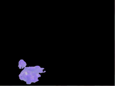 Nuclear segmentation of
 BloodImage_00001.jpg with color retained in the nucleus.
STOP: Before we return to the main text, try running the segmentation pipeline on a few different values of r_threshold, g_threshold, and b_threshold to see how they change the segmentation results. How could we quantify whether one collection of parameters is better than another? (You should use the values above the last time that you run the R pipeline so that your results will match those in future tutorials.)
