Software Tutorial: Training a Classifier on an Image Shape Space

Installing Weka

In this tutorial, we will apply the k-NN classifier to the post-PCA shape space of WBC nuclei images that we generated in the previous tutorial. To do so, we will need a statistical software framework that includes classification algorithms. There are a number of popular platforms available, but we will choose Weka, developed at the University of Waikato in New Zealand, since it is relatively light-weight and easy to get running quickly.

To install Weka, follow the instructions provided at the Weka wiki.

Converting a shape space file

To convert our current PCA pipeline coordinates to a format to be used in Weka, we need to convert the WBC_PCA.csv file that we produced in the previous tutorial and that contains the coordinates of every image in the post-PCA shape space into the arff format used by Weka. If you have not completed the previous tutorial, or you would like to skip to the next section of this tutorial, we provide the completed file for download here.

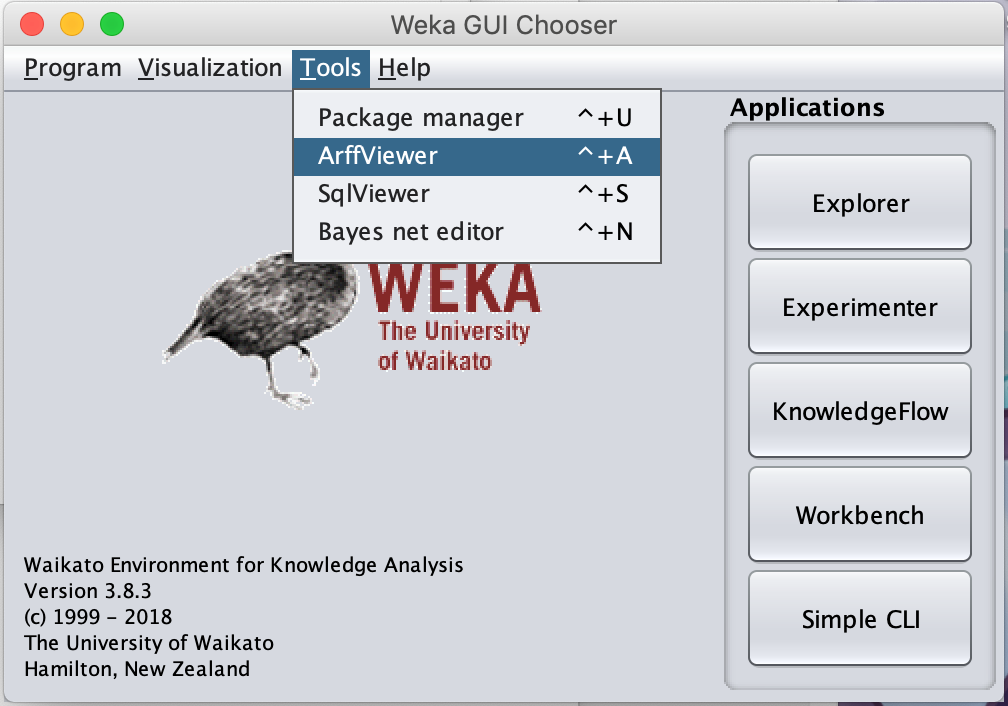
Open Weka and navigate to Tools --> ArffViewer.

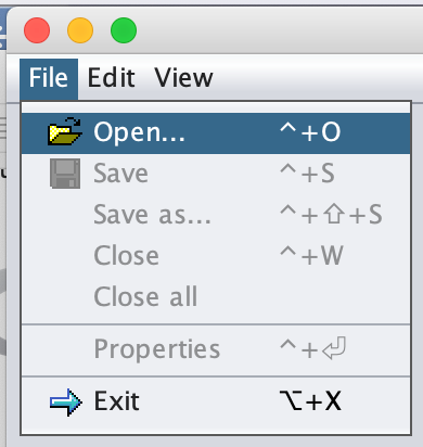
Then navigate to File --> Open.

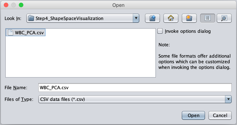
Change the Files of Type option to CSV data files.

Find (or download) the WBC_PCA.csv file in your Step4_Visualization folder and click Open.

Once all the data is loaded on screen, navigate to File --> Save as ….

Remove the .csv extension in the File Name field, and click Save.

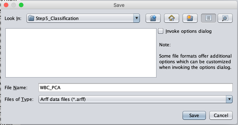
As a result, our PCA pipeline coordinates have now been converted to the file format that Weka accepts for further classification. This file should be saved as WBC_PCA.arff in the Step4_Visualization subfolder of the WBC_CellClass folder.

Now that we have the PCA dataset in the correct format, click Exit to return to the Weka home screen.

Running our first classifier

You should now be at the Weka GUI Chooser window that shows at the application’s startup. Under Applications, click Explorer to bring up the Weka Explorer window. This is the main window that we will use to run our classifier.

Next, we need to load our WBC_PCA.arff file that we just created. At the top left of the window, click Open file... Navigate to the location of your WBC_PCA.arff file (the default location would be Desktop/WBC_PCAPipeline/Step4_Visualization). When we do so, we should see the data loaded into the window, as shown in the figure below.

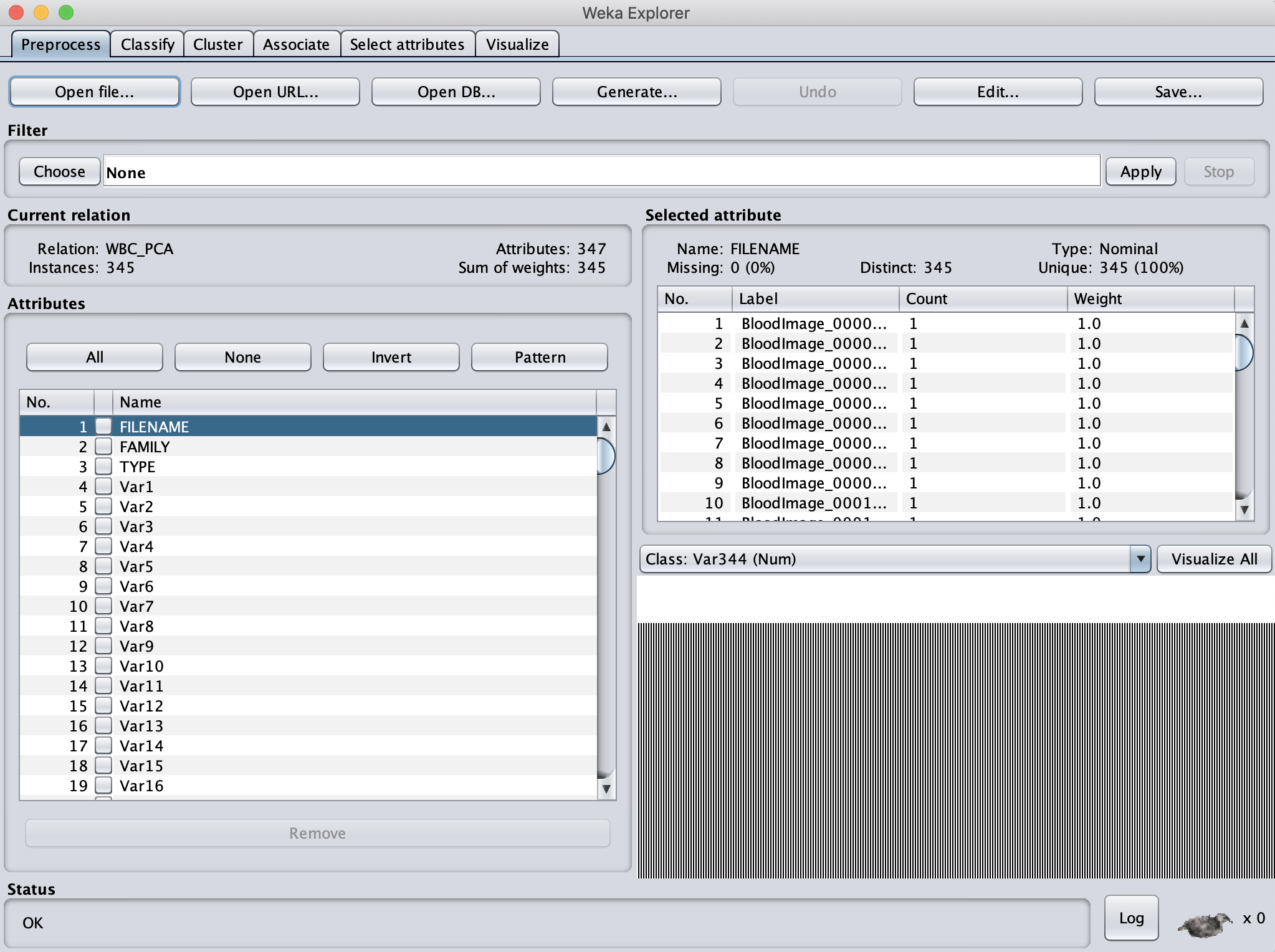
We want to ensure that Weka only considers the variables that are relevant for classifying the images by family. For this analysis, we won’t need the FILENAME name or the TYPE variables (if we were to include them, Weka would try to use them as one of the coordinates of our shape space vectors). So, click the checkboxes next to these two vectors, and click Remove to exclude them from consideration.

Let’s classify! Click the Classify tab at the top of the explorer window. Near the top of the window you will see a button that says Choose, with ZeroR next to it. This button will allow us to select our classifier.

If you’re curious what ZeroR means, it is the clown classifier from the main text that assigns every object to the class containing the most elements. Let’s not use this classifier! Instead, click Choose, which will bring up a menu of folders as shown below.

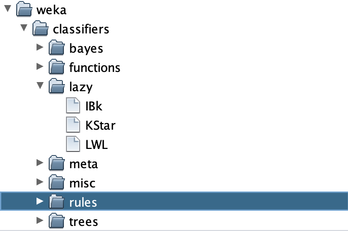
The k-NN classifer is contained under lazy > IBK. Select IBK, and you will be taken back to the explorer window, except that next to Choose you should now see IBK followed by a collection of parameters. The only parameter that we need for k-NN is the value of k (the number of nearest neighbors to consider when assigning a class to an object), which by default is set to 1 as indicated by -K 1.

Under Test Options, we see Cross-validation is selected, which is what we want. Let us leave the number of folds equal to 10, the default value.

Finally, beneath More options, we will see (Num) Var344. This is the variable that Weka will use to assign classes; rather, we would like Weka to classify objects by family. So, select this field, scroll up to the top, and select (Nom) FAMILY.

Note: Here, Num indicates a numeric variable, and Nom indicates a nominal variable (meaning that it corresponds to a name).

Now for the magic moment. Click Start. The classifier should run very quickly, and the results will show in the main window to the right and are reproduced below.

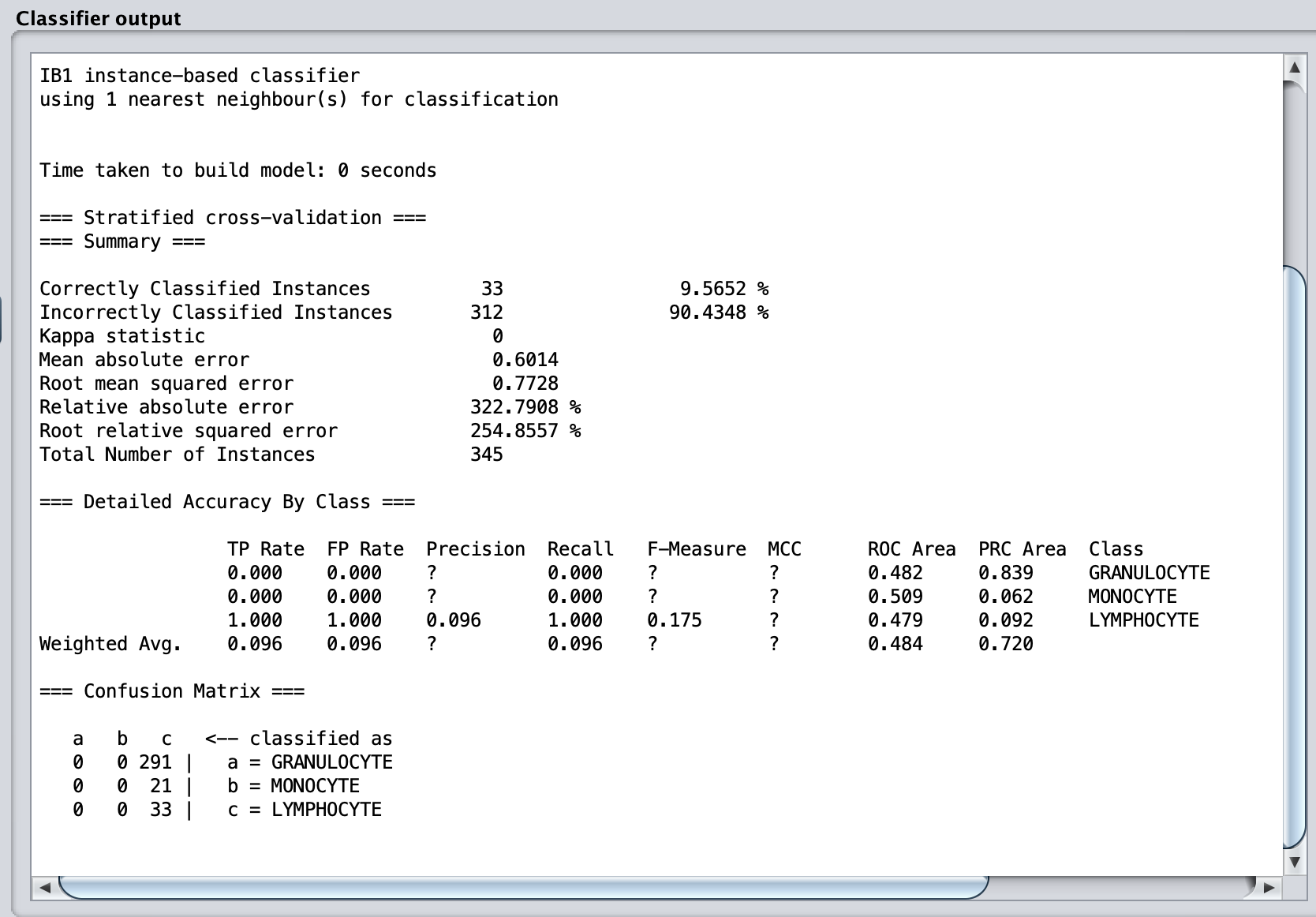
The results are horrible! Every image in our dataset has been assigned as a lymphocyte. What could have gone wrong?

Reducing the number of dimensions considered

Remember when we said that weird things happen in multi-dimensional space? The above result is one of those things. For some reason, every object in the dataset is closest to a lymphocyte. We could dig into the gritty details of the data to try and determine why this is the case, but instead, we will mutter something about the curse of dimensionality.

When we used CellOrganizer to build a shape space with PCA, it produced a hyperplane with 344 dimensions (one fewer than the total number of images), which is far more than we need. The good news is that one of the features of PCA is that if we would instead like a hyperplane with some smaller number of dimensions d, then we only need to consider the first d coordinates of every point in the space.

In our case, we will simply remove most of the variables under consideration by taking d = 20. To do so, click on the Preprocess tab. Under Attributes, select All, and then unselect FAMILY and the variables VAR1 through VAR20. Click Remove to ignore the other variables.

Removing variables is always counterintuitive to a three-dimensional mind, but let us see what happens when we run the classifier again. Click the Classify tab, and you will see that (Num) Var20 is selected as the variable to use for classification. Select (Nom) FAMILY and click Start. In our run, this produces the following confusion matrix in the output window.

Granulocyte	Monocyte	Lymphocyte
255	3	33
16	0	5
7	0	26

This is much better! The classifier seems to be performing particularly well on granulocytes. So, if removing some variables was a good thing, let’s remove a few more. Head back to Preprocess, remove Var16 through Var20, and run the classifier again. Our run yields the following updated confusion matrix.

Granulocyte	Monocyte	Lymphocyte
252	8	31
18	2	1
4	1	28

We are getting a little better! If we remove Var11 through Var15, you can verify that we obtain the following confusion matrix.

Granulocyte	Monocyte	Lymphocyte
259	9	23
14	6	1
5	2	26

In each step, our confusion matrix appears to be a little better, and the metrics that we introduced in the main text improve as well. In the Classifier output window, you can see that the accuracy has increased to 84.3%, while the weighted average of precision and recall over all three classes have increased to 0.857 and 0.843, respectively.

All this dimension reduction may make us wonder how far we should take it — should we reduce everything down to a single dimension? Yet if we remove Var6 through Var10, we see that our confusion matrix gets a little worse:

Granulocyte	Monocyte	Lymphocyte
261	13	17
13	8	0
16	2	17

And if we take the number of dimensions down to three, it gets a little worse still:

Granulocyte	Monocyte	Lymphocyte
257	15	19
16	5	0
20	0	13

We have therefore replicated an instance of a very deep fact in data science, which is that there is typically a “Goldilocks” value in the number of dimensions we should use for our PCA hyperplane, at which the algorithm is performing optimally. In the case of this WBC image dataset, that sweet spot value is around 10.

Note: If anything is still unclear about using Weka and exploring its output, Jen Golbeck made an excellent Youtube video that you may like to check out.

STOP: There are two other considerations that we should take into account: the value of k in our k-nearest neighbors approach (which has defaulted to 1) and the number of folds f used (which has defaulted to 10). We encourage you to continue running the k-NN classifier for a few different values of k and f (which can range from 2 to 365). What do you find? Does it match your intuition? And what happens if we try a different classifier entirely?

Subclassifying images by cell type

We classified our WBC images by family, but granulocytes further subdivide into three classes (basophils, eosinophils, and neutrophils). This means that we could just as well have classified images into five categories corresponding to cell type.

To do so, click the Preprocess tab at the top of the Weka explorer window. Click Open File again, and open your WBC_PCA.arff file. (It has not been modified by Weka.) This time, under Attributes, remove FILENAME, FAMILY, and the variables Var11 through Var344.

Then, click Classify, and again run k-NN with k = 1 and the number of folds equal to 10, making sure to select (Nom) TYPE as your variable to classify. As we return to the main text, we ask you to reflect on the results.

STOP: What are the accuracy, precision, and recall of this classifier? How does the confusion matrix compare to the one that we produced for three classes? From a biological perspective, why do you think that the algorithm is struggling?

Return to main text