 Leanpub
Introduction to artificial neuron models
The best known classification algorithms for WBC image analysis1 use a technique called deep learning. You have probably seen this term wielded with reverence, and so in this chapter’s conclusion, we will briefly explain what it means and how it can be applied to classification.
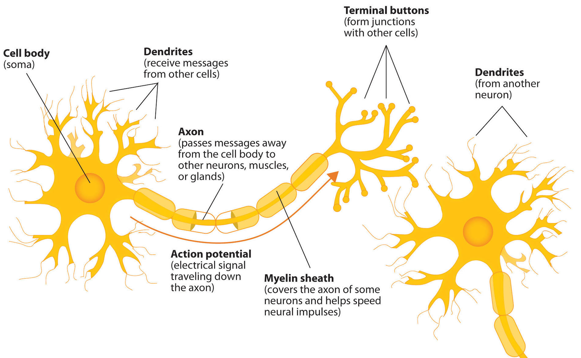
Neurons are cells in the nervous system that are electrically charged and that use this charge as a method of communication to other cells. As you are reading this text, huge numbers of neurons are firing in your brain as it processes the visual information that it receives. The basic structure of a neuron is shown in the figure below.
In 1943, Warren McCulloch (a neuroscientist) and Walter Pitts (a logician) devised an artificial model of a neuron that is now called a McCulloch-Pitts neuron.2 A McCulloch-Pitts neuron has a fixed threshold b and takes as input n binary variables x1, …, xn, where each of these variables is equal to either 0 or 1. The neuron outputs 1 if x1 + … + xn ≥ b; otherwise, it returns 0. If a McCulloch-Pitts neuron outputs 1, then we say that it fires.
The McCulloch-Pitts neuron with n equal to 2 and b equal to 2 is shown in the figure below. The only way that this neuron will fire is if both inputs x1 and x2 are equal to 1.
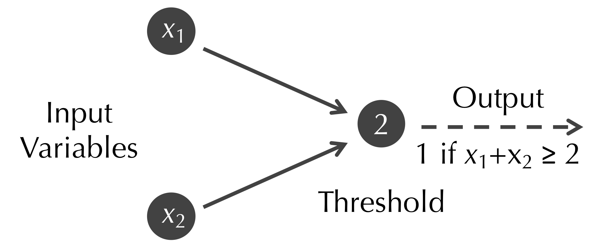
Note: The mathematically astute reader may have noticed that the output of the McCulloch-Pitts neuron in the figure above is identical to the logical proposition x1 AND x2, which explains why these neurons started as a collaboration between a neuroscientist and a logician.
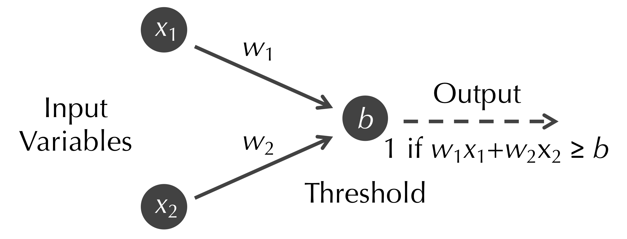
In 1958, Frank Rosenblatt generalized the McCulloch-Pitts neuron into a perceptron.3 This artificial neuron also has a threshold constant b and n binary input variables xi, but it also includes a collection of real-valued constant weights wi that are applied to each input variable. That is, the neuron will output 1 (fire) when the weighted sum w1 · x1 + w2 · x2 + … + wn · xn is greater than or equal to b.
Note: A McCulloch-Pitts neuron is a perceptron for which all of the wi are equal to 1.
For example, consider the perceptron shown in the figure below; we assign the weight wi to the edge connecting input variable xi to the neuron.
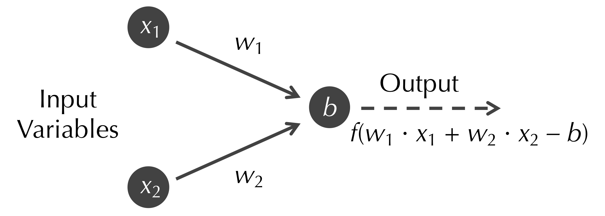
The modern concept of an artificial neuron, as shown in the figure below, generalizes the perceptron further in two ways. First, the input variables xi can have arbitrary decimal values (often, these inputs are constrained to be between 0 and 1). Second, rather than the neuron rigidly outputting 1 when w1 · x1 + w2 · x2 + … + wn · wn is greater than or equal to b, we subtract b from the weighted sum and pass the resulting value into a function f called an activation function; that is, the neuron outputs f(w1 · x1 + w2 · x2 + … + wn · wn). In this form of the neuron, b is called the bias of the neuron.
A commonly used activation function is the logistic function, f(x) = 1/(1 + e-x), shown in the figure below. Note that the output of this function ranges between 0 (when its input is very negative) and 1 (when its input is very positive).
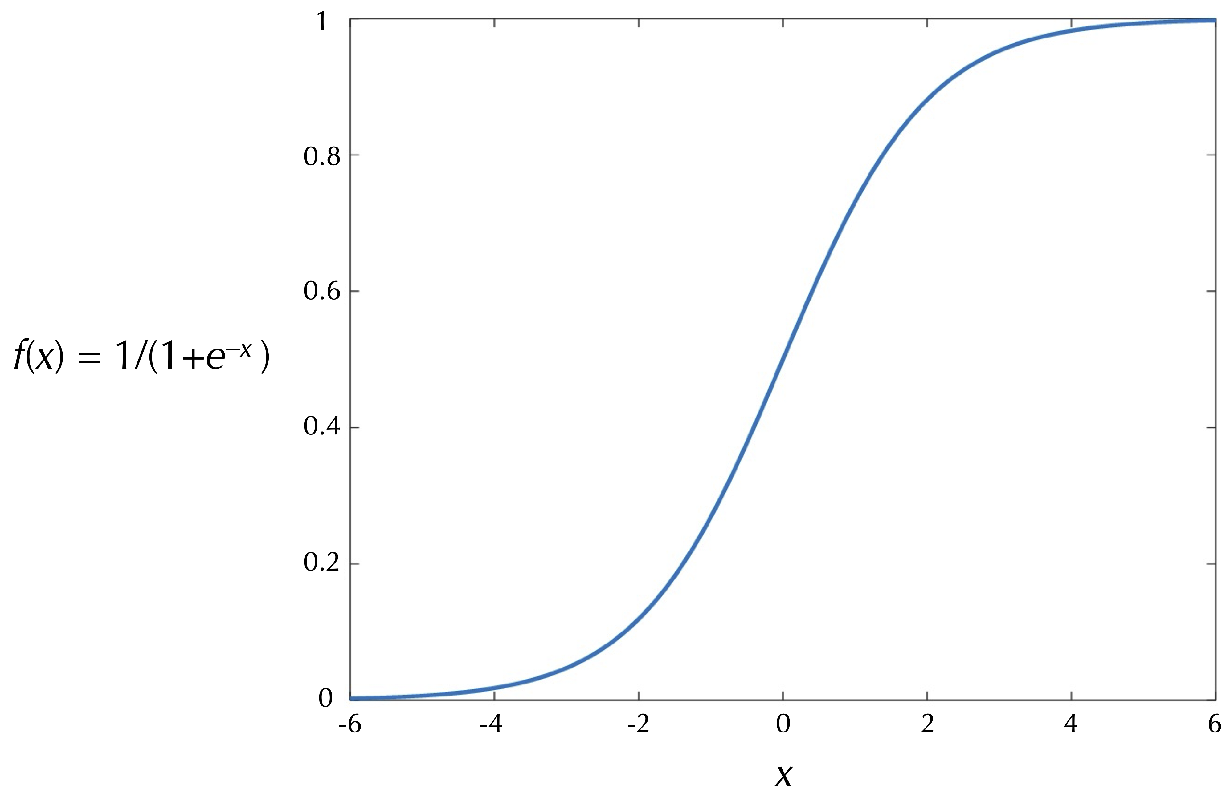
STOP: Because of its simplicity, researchers now often use a “rectifier” activation function: f(x) = max(0, x). What does the graph of this function look like? What is the activation function used by a perceptron, and how does it differ from the rectifier function?
Framing the WBC classification problem with neural networks
The outputs of mathematical functions can be used as inputs to other functions via function composition. For example, if f(x) = 2x-1, g(x) = ex, and h(x) = cos(x), then h(g(f(x))) = cos(e2x-1). Similarly, we can use artificial neurons as building blocks by linking them together, with the outputs of some neurons serving as inputs to other neurons. Linking neurons in this way produces a neural network such as the one shown in the figure below, which we will take time to explain.
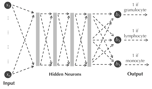
We have discussed converting each object x in a dataset (such as our WBC image dataset) into a feature vector (x1, x2, …, xn) representing each of the n feature values of x. In the figure above, these n variables of the data’s feature vectors become the n input variables of the neural network.
We typically then connect all the input variables to most or all of a collection of (possibly many) artificial neurons, called a hidden layer, which is shown for simplicity as a gray box in the figure above. If we have m artificial neurons in the hidden layer and n input variables, then we will have m bias constants as well as m · n weights, each one assigned to an edge connecting an input variable to a hidden layer neuron (all these edges are indicated by dashed edges in the figure above). Our model has quickly accumulated an enormous number of parameters!
The first hidden layer of neurons may then be connected as inputs to neurons in another hidden layer, which are connected to neurons in another layer, and so on. As a result, practical neural networks may have several hidden layers with thousands of neurons, each with their own biases, input weights, and even different activation functions. The most common usage of the term deep learning refers to solving problems using neural networks having several hidden layers; the discussion of the many challenges in designing neural networks for deep learning would fill an entire course.
The remaining question is what the output of our neural network should be. If we would like to apply the network to classify our data into k classes, then we typically will connect the final hidden layer of neurons to k output neurons. Ideally, if we know that a data point x belongs to the i-th class, then when we use the values of its feature vector as input to the network, we would like for the i-th output neuron to output a value close to 1, and for all other output neurons to output a value close to 0. For a neural network to correctly classify objects in our dataset, we must find such an ideal choice for the biases of each neuron and the weights assigned to input variables at each neuron — assuming that we have decided on which activation function(s) to use for the network’s neurons. We will now define quantitatively what makes a given choice of neural network parameters suitable for classification.
STOP: Say that a neural network has 100 input variables, three output neurons, and four hidden layers of 1000 neurons each. Say also that every neuron in one layer is connected as an input to every neuron in the next layer. How many bias parameters will this network have? How many weight parameters will this network have?
Defining the best choice of parameters for a neural network
In a previous lesson, we discussed how to assess the results of a classification algorithm like k-NN on a collection of data with known classes. To generalize this idea to our neural network classifier, we divide our data that have known classes into a training set and a test set, where the former is typically much larger than the latter. We then seek the choice of parameters for the neural network that “performs the best” on the training set, which we will now explain.
Each data point x in the training set has a ground truth classification vector c(x) = (c1, c2, …, ck),, where if x belongs to class j, then cj is equal to 1, and the other elements of c(x) are equal to 0. The point x also has an output vector o(x) = (o1, o2, …, ok), where for each i, oi is the output of the i-th output neuron in the network when x is used as the network’s input. The neural network is doing well at identifying the class of x when the classification vector c(x) is similar to the output vector o(x).
Fortunately, we have been using a method of comparing two vectors throughout this book. The RMSD between c(x) and o(x) measures how well the network classified data point x, with a value close to 0 representing a good fit. We can obtain a good measure of how well a neural network with given weight and bias parameters performs on a training set on the whole by taking the average RMSD between classification and output vectors over every element in the training set. We therefore would like to choose the biases and input weights for the neural network that minimize this average RMSD for all objects in the training set.
Once we have chosen a collection of bias and weight parameters for our network that perform well on the training set, we then assess how well these parameters performs on the test set. To this end, we can insert the feature vector of each test set object x as input into the network and consult the output vector o(x). Whichever i maximizes oi for this output vector becomes the assigned class of x. We can then use the metrics introduced previously in this module for quantifying the quality of a classifier to determine how well the neural network performs at classifying objects from the test set.
This discussion has assumed that we can easily determine the best choice of network parameters to produce a low mean RMSD between output and classification vectors for the training set. But how can we find this set of parameters in the first place?
Exploring a neural network’s parameter space
The typical neural network contains anywhere from thousands to billions of biases and input weights. We can think of these parameters as forming the coordinates of a vector in a high-dimensional space. From the perspective of producing low mean RMSD between output and classification vectors over a collection of training data, the vast majority of the points in this space (i.e., choices of network parameters) are worthless. In this vast landscape, a tiny number of these parameter choices will provide good results on our training set; even with substantial computational resources, finding one of these points is daunting.
The situation in which we find ourselves is remarkably similar to one we have encountered throughout this course, in which we need to explore a search space for some object that optimizes a function. We would therefore like to design a local search algorithm to explore a neural network’s parameter space.
As with ab initio structure prediction, we could start with a random choice of parameters, make a variety of small changes to the parameter values to obtain a set of “nearby” parameter vectors, and update our current parameter vector to the parameter vector from this set that produces the greatest decrease in mean RMSD between output and classification vectors. We then continue this process of making small changes to the current parameter vector until this mean RMSD stops decreasing. This local search algorithm is similar to the most popular approach for determining parameters for a neural network, called gradient descent.
STOP: What does a local minimum mean in the context of neural network parameter search?
Just as we run ab initio structure prediction algorithms using many different initial protein conformations, we should run gradient descent for many different sets of randomly chosen initial parameters. In the end, we take the choice of parameters minimizing mean RMSD over all these trials.
Note: If you find yourself interested in deep learning and would like to learn more, check out the excellent Neural Networks and Deep Learning online book by Michael Nielsen.
Neural network pitfalls, Alphafold, and final reflections
Neural networks are wildly popular, but they have their own issues. Because we have so much freedom for how the neural network is formed, it is challenging to know a priori how to design an “architecture” for how the neurons should be connected to each other for a given problem.
Once we have decided on an architecture, the neural network has so many bias and weight parameters that even with access to a supercomputer, it may be difficult to find values for these parameters that perform even reasonably well on the training set; the situation of having parameters with high RMSD for the training set is called “underfitting”. Even if we build a neural network having low mean RMSD for the training set, the neural network may perform horribly on the test set, which is called “overfitting” and offers yet another instance of the curse of dimensionality.
Despite these potential concerns with neural networks, they are starting to show promise of making significant progress in solving biological problems. AlphaFold, which we introduced when discussing protein folding, is powered by neural networks that contain 21 million parameters. Yet although AlphaFold has revolutionized the study of protein folding, just as many problems exist for which neural networks are struggling to make progress over existing methods. Biology largely remains, like the environment of a lonely bacterium, an untouched universe waiting to be explored.
Thank you!
If you are reading this, and you’ve made it through our entire course, thank you for joining us on this journey! We are grateful that you gave your time to us, and we wish you the best on your educational journey. Please don’t hesitate to contact us if you have any questions, feedback, or would like to leave us a testimonial; we would love to hear from you.
-
Habibzadeh M, Jannesari M, Rezaei Z, Baharvand H, Totonchi M. Automatic white blood cell classification using pre-trained deep learning models: ResNet and Inception. Proc. SPIE 10696, Tenth International Conference on Machine Vision (ICMV 2017), 1069612 (13 April 2018). Available online ↩
-
McCulloch WS, Pitts WS 1943. A Logical calculus of the ideas Immanent in nervous activity. The bulletin of mathematical biophysics (5): 115–133. Available online ↩
-
Rosenblatt M 1958. The perceptron: a probabilistic model for information storage and organization in the brain. Psychological review 65 (6): 386. ↩
