 Leanpub
In a previous tutorial, we segmented and binarized a collection of WBC images. If you completed that tutorial, then you should see those images as a collection of .tiff files in your BWImgs_1 folder inside your WBC_PCAPipeline/Data directory.
We are now ready to use CellOrganizer to build a shape space of these images and then apply PCA to the resulting shape vectors in order to reduce the dimension of the dataset.
Note: This version of the tutorial is modified to use the Docker implementation of CellOrganizer rather than the (standard) MATLAB implementation. We created this alternative version primarily for Windows users to allow them to run CellOrganizer. Those who are running a Mac/Linux machine may prefer to follow the original tutorial. Note that MATLAB is still required for this version of the tutorial.
Necessary Software
We will need to install Docker in order to use this version of CellOrganizer. To do so, follow the instructions here. For Windows users, we also recommend installing a UNIX-like terminal such as Git Bash, which can be downloaded as part of Git for Windows.
Note: In order to get Docker to run, it may be necessary for Windows users to set up the Windows Subsystem for Linux. Also, depending on the computer, it may be necessary to modify the computer’s BIOS settings and enable virtualization technology in order to get Docker to run. Consult the help sections on WSL and virtualization for more details.
Running CellOrganizer for Docker
CellOrganizer for Docker is accessed via a Jupyter notebook server interface. To get started, first ensure that Docker is running by launching the Docker Desktop app. Next, follow the instructions here to start the server.
Note: To execute the run.sh script from the instructions above, first navigate to the folder where you saved the file using Git Bash, and execute the command bash ./run.sh. For example, if you saved the file onto your desktop, you would first type in cd ~/Desktop, and then bash ./run.sh to run the bash script.
The output from running the commands in the instructions above is shown below. To access the Jupyter notebook server, copy the URL shown at the bottom of the output (highlighted below).
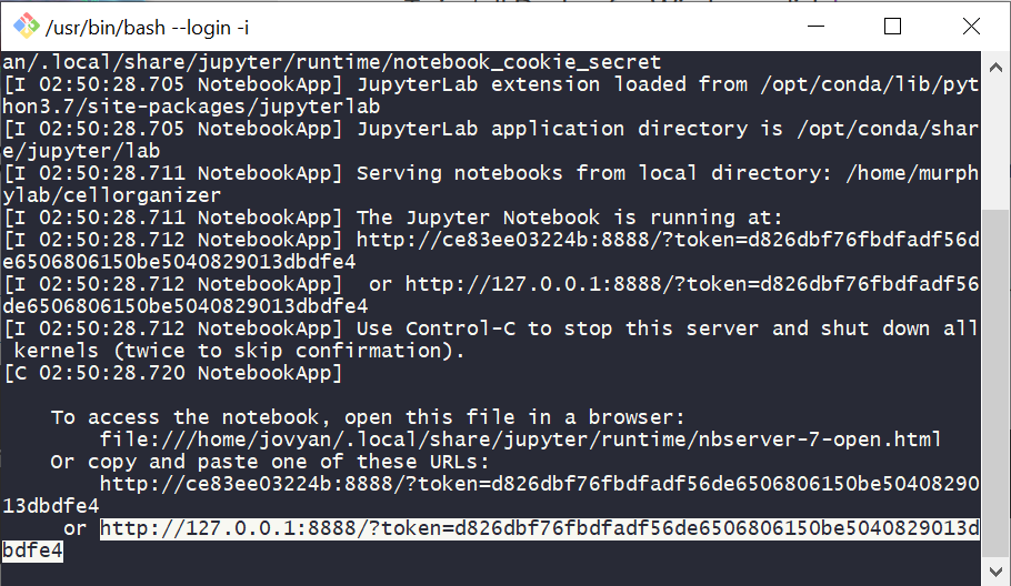
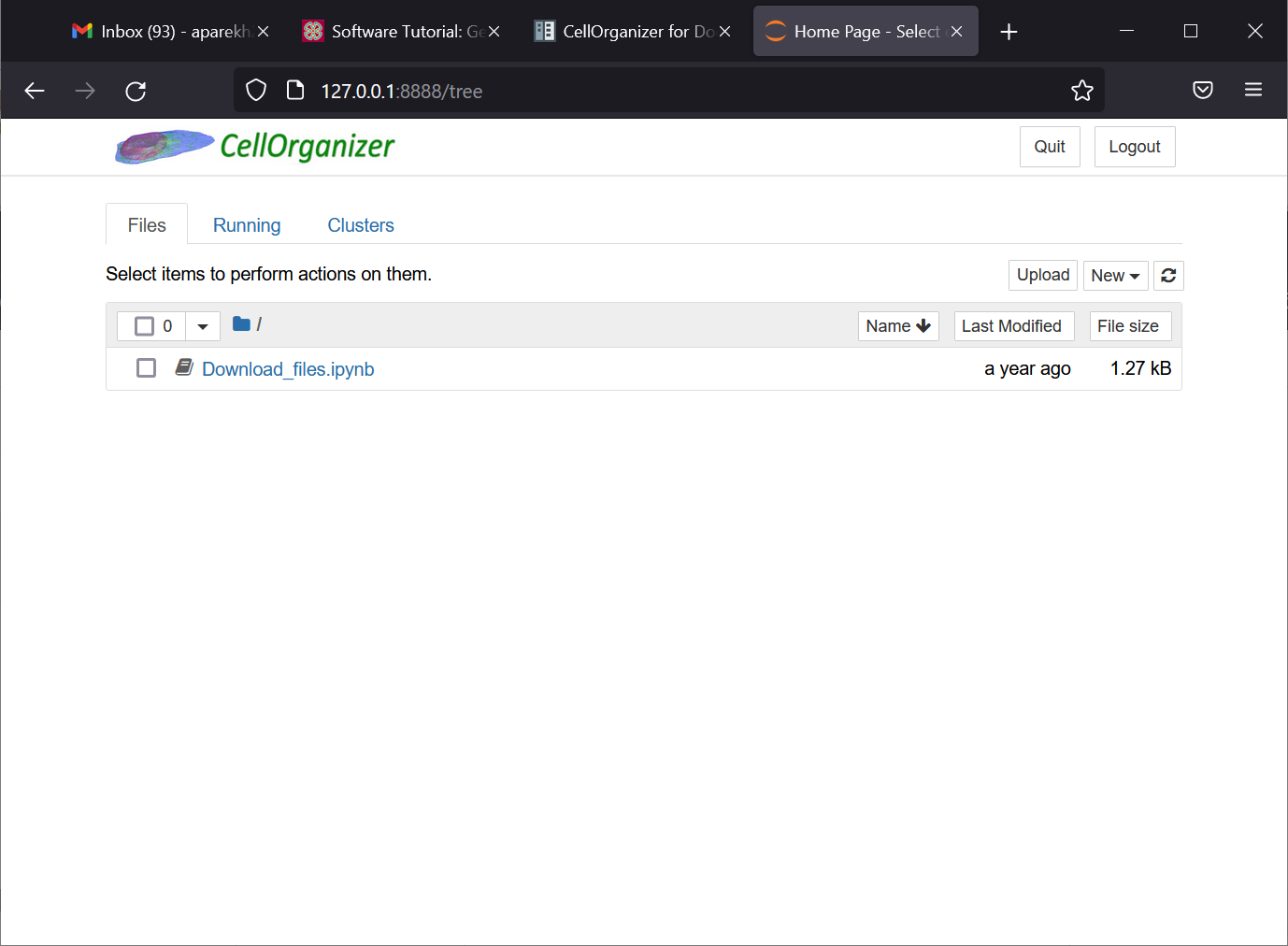
Open a web browser, and navigate to the URL you copied above. This will open the Jupyter notebook server in your browser, which contains all of the software needed to run CellOrganizer and create our model.
Next, we need to upload our images to the server so that they can be fed as input to the CellOrganizer model. The most straightforward way to do this would be to upload our WBC_PCAPipeline/Data/BWImgs_1 folder onto the server, but unfortunately we can only upload individual files onto the server. Fortunately, there is a simple workaround - Jupyter notebooks allows us to upload zipped folders, so we can instead upload a zipped folder onto the server which contains all of our images.
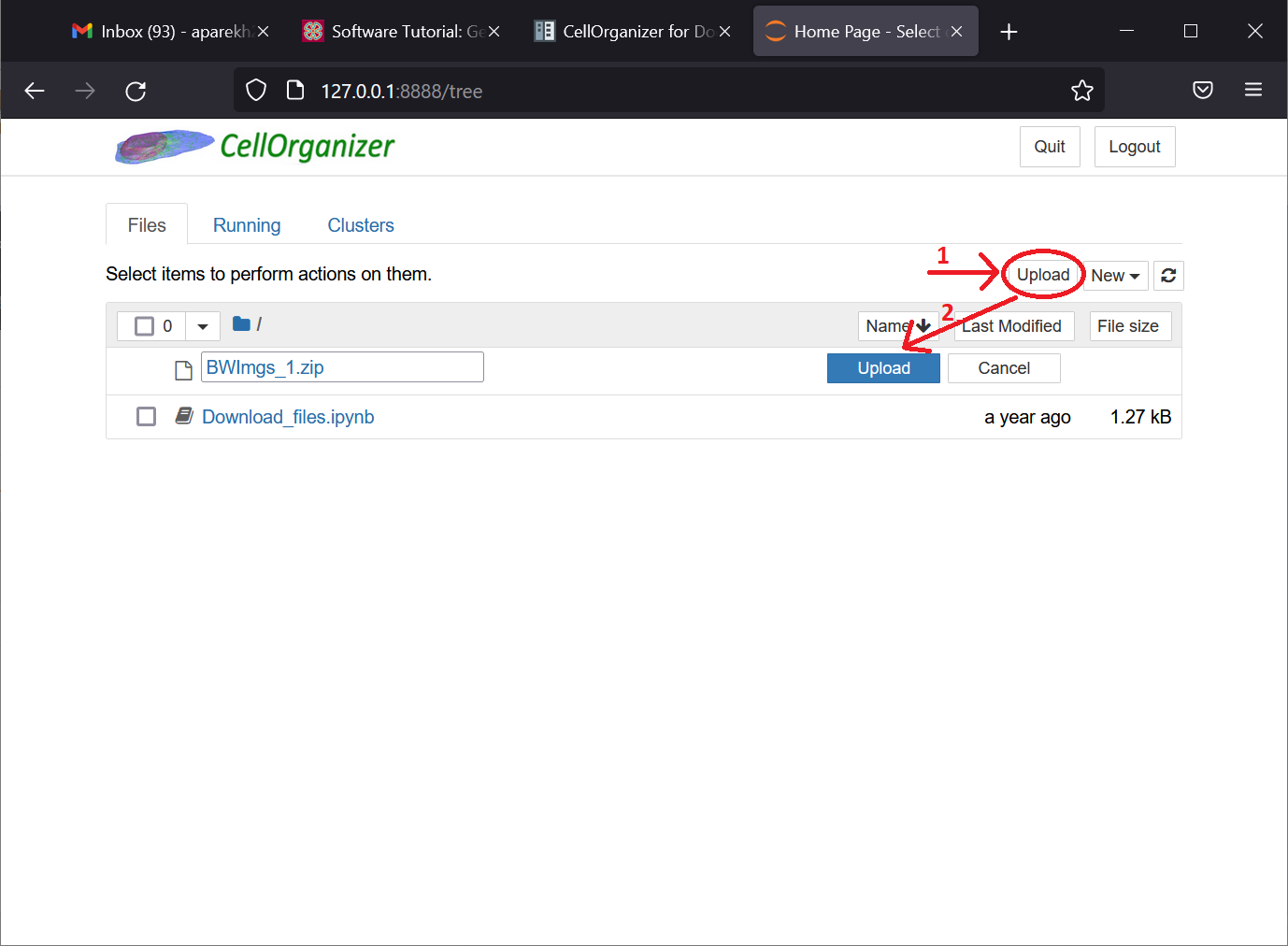
First, compress your BWImgs_1 folder into a .zip file by right-clicking on the folder in File Explorer and selecting send to > Compressed (zipped) folder. Next, click the upload button near the top-right corner of the Jupyter notebook screen, and double-click on the BWImgs_1.zip file you just created. Then, click the upload button next to the newly added folder.
We are now ready to start using CellOrganizer! Create a new IPython notebook on the server named WBC_PCA.ipynb, and enter the following code into a code cell. We will not do a line-by-line walkthrough of the code here, but feel free to compare it with the corresponding MATLAB code contained in Step3_ModelGeneration/WBC_PCAModel.m.
! unzip BWImgs_1  # unzip folder - the ! specifies a UNIX command (not python)

# import CellOrganizer functions
from cellorganizer.tools import img2slml, slml2info

import os
import sys

# Specify model options for CellOrganizer
options = {'verbose': True,
           'debug': False,
           'display': False,
           'model.name': 'WBC_PCA',
           'train.flag': 'framework',
           'nucleus.class': 'framework',
           'nucleus.type': 'pca',
           'cell.class': 'framework',
           'cell.type': 'pca',
           'skip_preprocessing': True,

           # Latent Dimension for the Model
           'latent_dim': 15,

           # No idea what this is for
           'masks': [],

           'model.resolution': [0.049, 0.049],
           'model.filename': 'WBC_PCA.xml',
           'model.id': 'WBC_PCA',

           # Set nuclei and cell model name
           'nucleus.name': 'WBC_NUC',
           'cell.model': 'WBC_CELL',

           'documentation.description': 'Trained using demo2D08 from CellOrganizer.'}

dimensionality = '2D'

# Set path to the binarized segmented images
directory = os.path.join('.', 'BWImgs_1')
dna = [os.path.join(directory, 'bw*.tiff')]
cellm = [os.path.join(directory, 'bw*.tiff')]

# Create the shape space model
img2slml(dimensionality, dna, cellm, [], options)

# img2slml results saved in a MATLAB data file if command run successfully.
print("Model output saved successfully:", "WBC_PCA.mat" in os.listdir())
The results of running the Python code above will be a new file called WBC_PCA.mat stored on the Jupyter notebook server. Download the file onto your own local computer, and store it in the folder WBC_PCAPipeline/Step3_ModelGeneration.
Next, start MATLAB, and set the MATLAB path by clicking the button indicated below, and navigating to your WBC_PCAPipeline/Step3_ModelGeneration folder.
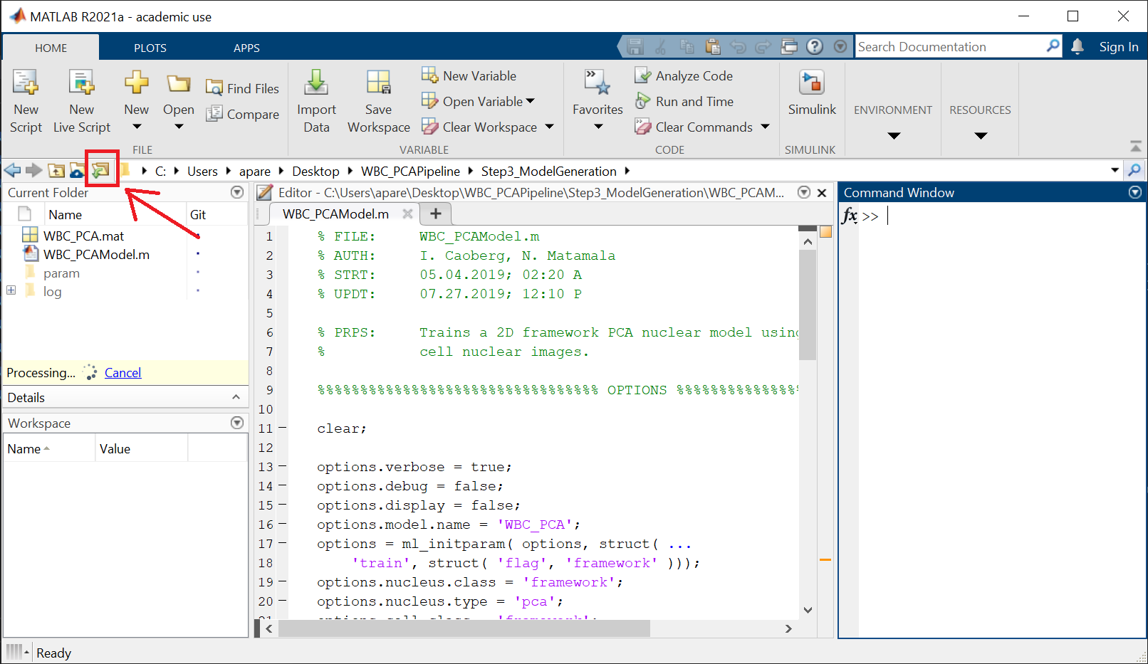
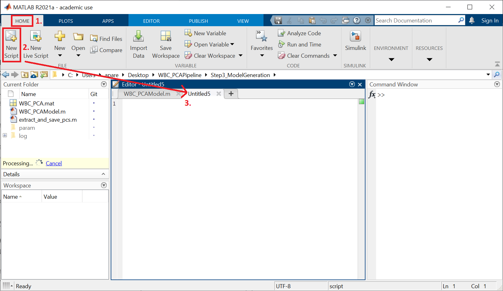
Once the path is set, navigate to the Home pane at the top of your MATLAB window, and click on the New Script button. This will open up a new script in your editor window.
Enter the following lines of MATLAB code into the newly opened file, which extract and save the principal components from your model to a .csv file:
load( [pwd filesep 'WBC_PCA.mat'] );
scr = array2table(model.nuclearShapeModel.score);
lbls = readtable('../Data/WBC_Labels.csv');
mtrx = [lbls scr];
writetable(mtrx, '../Step4_Visualization/WBC_PCA.csv');
Save the file as extract_and_save_pcs.m in your Step3_ModelGeneration folder. Next, in the MATLAB command window, type in
extract_and_save_pcs
This will run the script, and the result will be a new file, WBC_PCA.csv, saved to the folder Step4_Visualization. This file contains the shape vector of each image after PCA has been applied.
Note: If you use this file as input for the next tutorial, then you will obtain very slightly different results from those in the text. The reasons why these results do not match are not clear but the conclusions will remain the same.
That’s it! You can now follow along the remainder of the tutorial, in which we visualize the post-PCA shape space.
