Software Tutorial: Implementing the Repressilator

Note: We are currently in the process of updating this tutorial to the latest version of MCell, CellBlender, and Blender. This tutorial works with MCell3, CellBlender 3.5.1, and Blender 2.79. Please see a previous tutorial for a link to download these versions.

In this tutorial, we will use CellBlender to build a particle-based simulation implementing a repressilator. First, load the CellBlender_Tutorial_Template.blend file from the Random Walk Tutorial and save a copy of the file as repressilator.blend. You may also download the completed tutorial file here.

Then go to CellBlender > Molecules and create the following molecules:

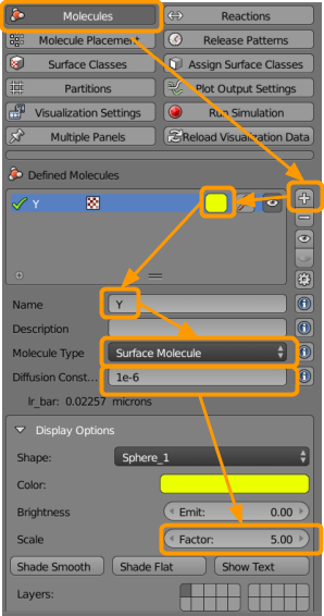
1. Click the + button.
2. Select a color (such as yellow).
3. Name the molecule Y.
4. Select the molecule type as Surface Molecule.
5. Add a diffusion constant of 1e-6.
6. Up the scale factor to 5 (click and type “5” or use the arrows).

Repeat the above steps to make sure that the following molecules are all entered with the appropriate parameters.

Molecule Name	Molecule Type	Diffusion Constant	Scale Factor
X	Surface	4e-5	5
Y	Surface	4e-5	5
Z	Surface	4e-5	5
HiddenX	Surface	3e-6	3
HiddenY	Surface	3e-6	3
HiddenZ	Surface	3e-6	3
HiddenX_off	Surface	1e-6	3
HiddenY_off	Surface	1e-6	3
HiddenZ_off	Surface	1e-6	3

Now go to CellBlender > Molecule Placement to establish molecule release sites by following these steps:

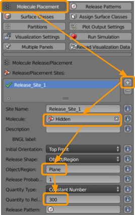
1. Click the + button.
2. Select or type in the molecule X.
3. Type in the name of the Object/Region Plane.
4. Set the Quantity to Release as 150.

Repeat the above steps to make sure the following molecules are entered with the appropriate parameters as shown below.

Molecule Name	Object/Region	Quantity to Release
X	Plane	150
HiddenX	Plane	100
HiddenY	Plane	100
HiddenZ	Plane	100

Next go to CellBlender > Reactions to create the following reactions:

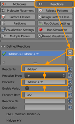
1. Click the + button.
2. Under reactants, type HiddenX’ (note the apostrophe).
3. Under products, type HiddenX’ + X’.
4. Set the forward rate as 2e3.

Repeat the above steps for the following reactions, ensuring that you have the appropriate parameters for each reaction.

Note: Some molecules require an apostrophe or a comma. This represents the orientation of the molecule in space and is very important to the reactions!

Reactants	Products	Forward Rate
HiddenX’	HiddenX’ + X’	2e3
HiddenY’	HiddenY’ +Y’	2e3
HiddenZ’	HiddenZ’ + Z’	2e3
X’ + HiddenY’	HiddenY_off’ + X,	6e2
Y’ + HiddenZ’	HiddenZ_off’ + Y,	6e2
Z’ + HiddenX’	HiddenX_off’ + Z,	6e2
HiddenX_off’	HiddenX’	6e2
HiddenY_off’	HiddenY’	6e2
HiddenZ_off’	HiddenZ’	6e2
X’	NULL	6e2
Y’	NULL	6e2
Z’	NULL	6e2
X,	X’	2e2
Y,	Y’	2e2
Z,	Z’	2e2

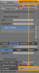
Go to CellBlender > Plot Output Settings to build a plot as follows:

1. Click the + button.
2. Set the molecule name as X.
3. Ensure World is selected.
4. Ensure Java Plotter is selected.
5. Ensure One Page, Multiple Plots is selected.
6. Ensure Molecule Colors is selected.

Repeat the above steps for the following molecules.

Molecule Name	Selected Region
X	World
Y	World
Z	World

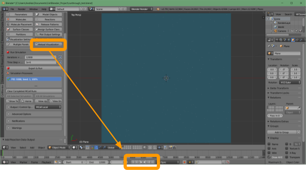
We are now ready to run our simulation. Go to CellBlender > Run Simulation and select the following options:

1. Set the number of iterations to 120000.
2. Ensure the time step is set as 1e-6.
3. Click Export & Run.

Once the simulation has run, visualize the results of the simulation with CellBlender > Reload Visualization Data.

Now go back to CellBlender > Plot Output Settings and scroll to the bottom to click Plot.

Does the plot that you obtain look like a biological oscillator? As we return to the main text, we will interpret this plot and then see what will happen if we suddenly shift the concentration of one of the particles. Will the system still retain its oscillations?

Return to main text