 Leanpub
Simulating transcriptional regulation with a reaction-diffusion model
Theodosius Dobzhansky famously wrote that “nothing in biology makes sense except in the light of evolution.”1 In the spirit of this quotation, some evolutionary reason must explain the presence of the large number of negatively autoregulating E. coli transcription factors that we identified in the previous lesson. Our goal is to use biological modeling to establish this justification.
We will simulate a “race” to the steady state, or equilibrium, concentration of a transcription factor Y in two cells, shown in the figure below. In the first cell, a transcription factor X activates Y; in the second cell, Y also negatively autoregulates. Our premise is that the cell that reaches the steady state faster can respond more quickly to its environment and is therefore more fit for survival.
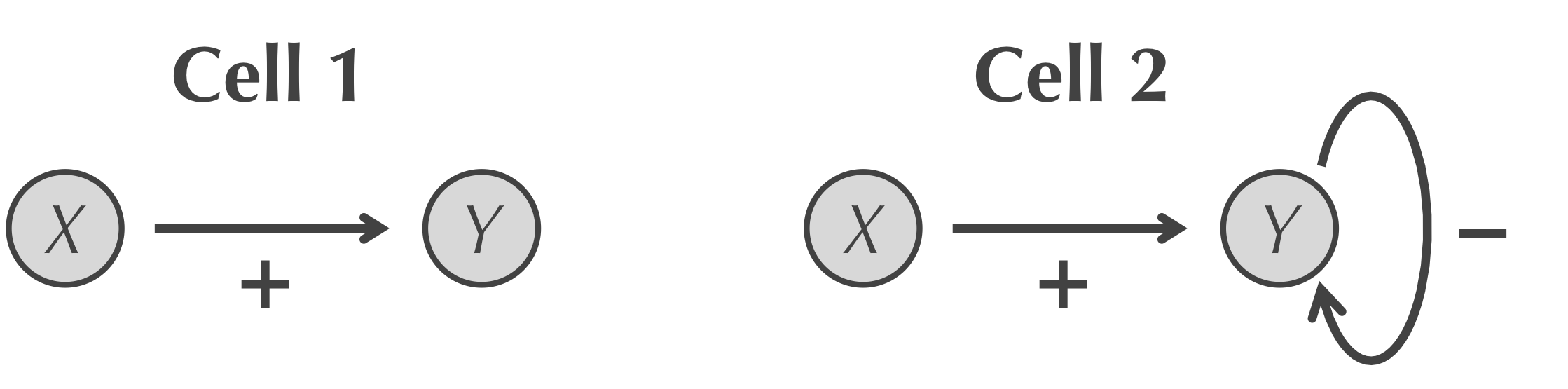 The two cells that we wish to simulate. In the first cell (left), X only activates Y; in the second cell (right), Y also negatively autoregulates.
We will simulate these two cells using a reaction-diffusion model analogous to the one introduced in the prologue. For our new model, the “particles” represent the two transcription factors X and Y.
We begin with the first cell. To simulate X activating Y, we use the reaction X → X + Y. In a given interval of time, there is a constant underlying probability related to the reaction rate that any given X particle will spontaneously form a new Y particle.
We should also account for the fact that proteins are degraded over time by enzymes called proteases. The typical protein’s concentration will be degraded by 20 to 40 percent in an hour, but transcription factors degrade even faster, with each one lasting only a matter of minutes.2 Protein degradation is an important feature of cellular design, as it allows the cell to remove a protein after increasing that protein’s concentration in response to some environmental change.
To model the degradation of Y, we add a “kill” reaction that removes Y particles at some rate. We will initialize our simulation with no Y particles and the X concentration at steady state; since X is being produced at a rate that exactly balances its degradation rate, we will not need to add reactions to the model simulating the production or degradation of X.
To complete the model of the first cell, diffusion of the X and Y particles is not technically necessary because no reaction in our model requires the collision of two or more particles. However, for the sake of biological correctness, we will allow both X and Y particles to diffuse through the system at the same rate.
STOP: What chemical reaction could be used to simulate the negative autoregulation of Y?
The model of the second cell will inherit all of the reactions from the first cell (with the same reaction rates) while adding negative autoregulation of Y, which we will model using the reaction 2Y → Y. That is, when two Y particles collide, there is some probability related to the reaction rate that one of the particles serves to remove the other, which mimics the process of a transcription factor turning off another copy of itself during negative autoregulation.
To recap, both simulated cells will include an initial concentration of X at steady state, diffusion of X and Y, removal of Y, and the reaction X → X + Y. The second simulation, which includes negative autoregulation of Y, will add the reaction 2Y → Y. You can explore these simulations in the following tutorial.
Note: Although we are using a particle-based model to mimic regulation, it does not implement specific chemical reactions. In reality, gene regulation is a complicated chemical process that involves a great deal of molecular machinery. The purpose of the model is to strip away the irrelevant and retain the essence of what is being modeled.
Ensuring a mathematically controlled comparison
If you followed the above tutorial, then you were likely disappointed in the second cell and its negative autoregulating transcription factor Y. shows a plot over time of the concentration of Y particles in the two simulated cells, using yellow for the first cell and blue for the second cell.
 A plot of the concentration of Y particles over time across two simulations. In the first cell (red), we only have activation of Y by X, whereas in the second cell (yellow), we keep all parameters fixed but add a reaction simulating the negative autoregulation of Y.
By allowing Y to slow its own transcription, we wound up with a simulation in which the final concentration of Y was lower. How could negative autoregulation possibly be useful?
The solution to this quandary is that the model we built was not a fair comparison between the two systems. In particular, the two simulations converge to approximately the same steady state concentration of Y, since achieving this concentration represents the cell’s response to some stimulus. Ensuring this equal footing for the two simulations is called a mathematically controlled comparison.3
STOP: How can we change the parameters of our models to obtain a mathematically controlled comparison of the two simulated cells?
We should keep a number of parameters constant across the two simulations because they are unrelated to regulation: the diffusion rates of X and Y, the number of initial particles X and Y, and the degradation rate of Y. With these parameters fixed, the only way that the final steady state concentration of Y can be the same in the two simulations is if we increase the rate at which the reaction X → X + Y takes place in the simulation of the second cell. The following tutorial adjusts this rate parameter to ensure a mathematically controlled comparison.
An evolutionary basis for negative autoregulation
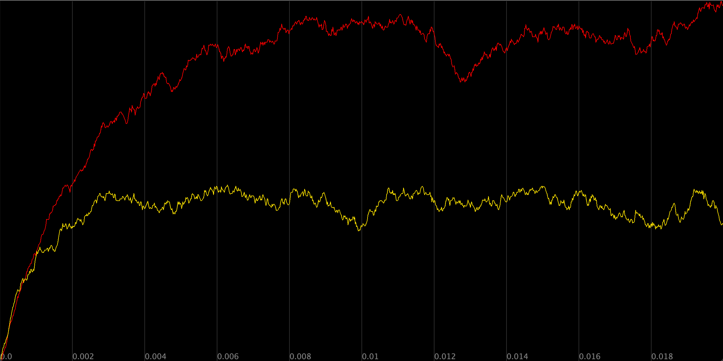
The figure below plots the concentration over time of Y particles for the two simulated cells after ensuring a mathematically controlled comparison, in which the rate of the reaction X → X + Y has been increased in the second cell. This figure shows that the two simulated cells now have approximately the same steady state concentration of Y. However, the second cell reaches this concentration faster; that is, its response time to the external stimulus that caused an increase in the production of Y is shorter.
 A comparison of the concentration of Y particles across the same two simulations from the previous figure. This time, in the second simulation (yellow), we increase the rate of the reaction X → X + Y. As a result, the two simulations have approximately the same steady state concentration of Y, and the simulation that includes negative autoregulation reaches steady state more quickly.
The above plots also provide evidence of why negative autoregulation may have evolved. The simulated cell that includes negative autoregulation wins the “race” to a steady state concentration of Y, and so we can conclude that this cell is more fit for survival than one in which Y does not negatively autoregulate. Uri Alon4 has proposed an excellent analogy of a negatively autoregulating transcription factor as a sports car that has both a powerful engine (corresponding to the higher rate of the reaction producing Y) and sensitive brakes (corresponding to negative autoregulation slowing the production of Y to reach equilibrium quickly).
In this lesson, we have seen that particle-based simulations can be powerful for justifying why a network motif is prevalent. What are some other commonly occurring network motifs in transcription factor networks? And what evolutionary purposes might they serve?
-
Dobzhansky, Theodosius (March 1973), “Nothing in Biology Makes Sense Except in the Light of Evolution”, American Biology Teacher, 35 (3): 125–129, JSTOR 4444260) ↩
-
Goodsell, David (2009), The Machinery of Life. Copernicus Books. ↩
-
Savageau, M (1976). Biochemical systems analysis: A study of function and design in molecular biology. Addison Wesley. ↩
-
Alon, Uri. An Introduction to Systems Biology: Design Principles of Biological Circuits, 2nd Edition. Chapman & Hall/CRC Mathematical and Computational Biology Series. 2019. ↩
