 Leanpub
Note: We are currently in the process of updating this tutorial to the latest version of MCell, CellBlender, and Blender. This tutorial works with MCell3, CellBlender 3.5.1, and Blender 2.79. Please see a previous tutorial for a link to download these versions.
In this tutorial, we will use CellBlender to adapt our simulation from the tutorial on negative autoregulation into a mathematically controlled simulation.
First, open the file NAR_comparison.blend from the negative autoregulation tutorial and save a copy of the file as NAR_comparison_equal.blend. You may also download the completed tutorial files here.
Now go to CellBlender > Reactions to scale up the simple regulation reaction in the negative autoregulation simulation as follows: for the reaction X2’ -> X2’ + Y2’, change the forward rate from 4e2 to 4e3.
Next go to CellBlender > Run Simulation and ensure that the following options are selected:

- Set the number of iterations to
20000. - Ensure the time step is set as
1e-6. - Click
Export & Run.
Click CellBlender > Reload Visualization Data. You have the option of watching the animation within the Blender window by clicking the play button at the bottom of the screen.
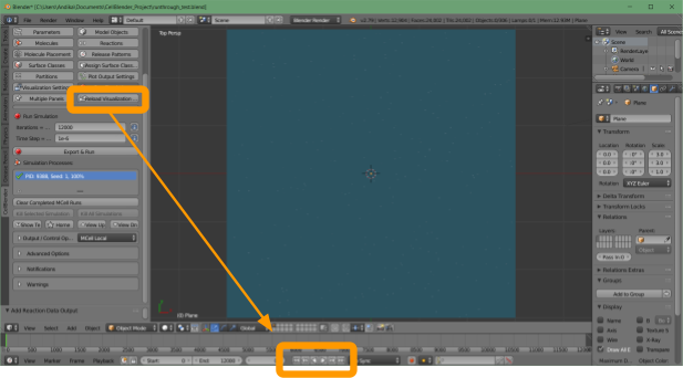
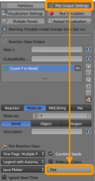
Now go back to CellBlender > Plot Output Settings and scroll to the bottom to click Plot; this should produce a plot. How does your plot
Save your file before returning to the main text, where we will interpret the plot produced to see if we were able to obtain a mathematically controlled simulation and then interpret the result of this simulation from an evolutionary perspective.
