 Leanpub
Feedforward loops
In the previous lesson, we saw that negative autoregulation can be used to lower the response time of a protein to an external stimulus. But the cell can only use autoregulation to respond quickly if the autoregulated protein is itself a transcription factor. Only about 300 of the 4,400 total E. coli proteins are transcription factors1. How can the cell speed up the manufacture of a protein that is not a transcription factor?
The answer lies in another transcription factor network motif called the feedforward loop (FFL). An FFL, shown in the figure below, is a network substructure in which X is connected to both Y and Z, and Y is connected to Z. Calling the FFL motif a “loop” is a misnomer. Rather, it is a small network structure with two paths from X to Z; one via direct regulation of Z by X, and another with an intermediate transcription factor Y. Note that X and Y must be transcription factors because they have edges leading out from them, but Z does not have to be a transcription factor (and typically is not).
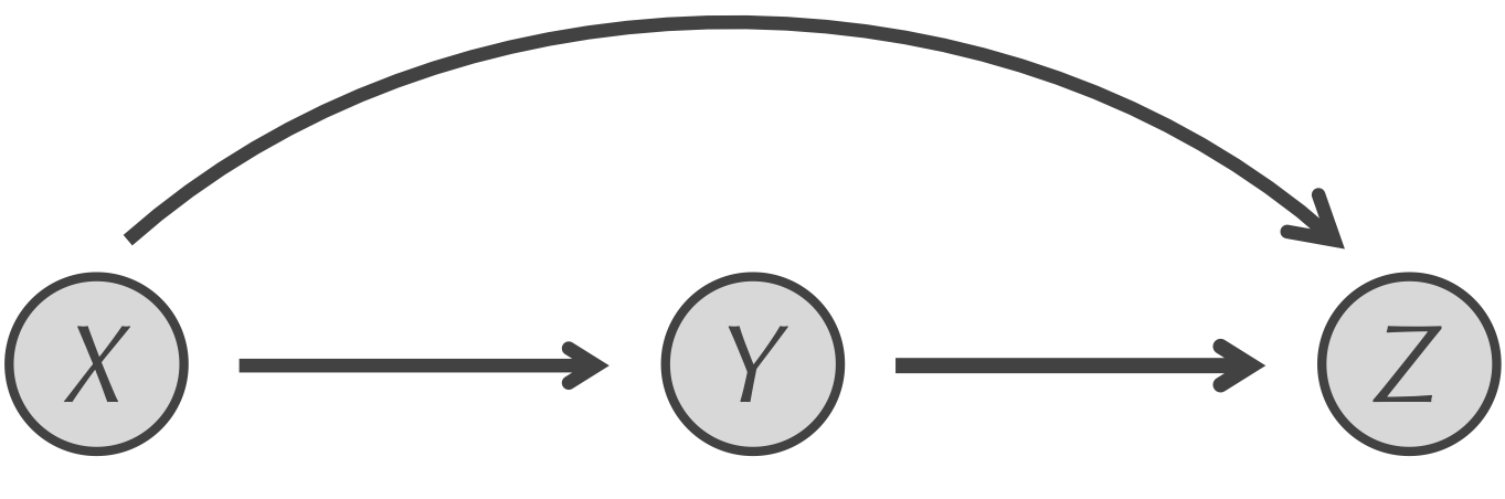 The FFL motif. X regulates both Y and Z, and Y regulates Z.
There are 42 FFLs in the transcription factor network of E. coli2, of which five have the structure below, in which X activates Y, X activates Z, and Y represses Z. This specific form of the FFL motif is called a type-1 incoherent feedforward loop and will be our focus for the rest of the module.
STOP: How could we simulate a type-1 incoherent feedforward loop with a particle-based reaction-diffusion model akin to the simulation that we used for negative autoregulation? What would we compare this simulation against?
 The incoherent feed-forward loop network motif. X activates Y and Z (the associated edges are labeled with “+”), while Y represses Z (the associated edge is labeled with “-“).
Modeling a type-1 incoherent feedforward loop
As we did for negative autoregulation, we will simulate two cells and examine the concentration of a particle of interest, which in this case will be Z. The first cell will have a simple activation of Z by X; we will assume that X starts at its steady state concentration and that Z is produced by the reaction X → X + Z and removed by a degradation reaction.
The second cell will include both of these reactions in addition to the reaction X → X + Y to model the activation of Y by X, along with the new reaction Y + Z → Y to model the repression of Z by Y. Because Y and Z are being produced from a reaction, we will also have degradation reactions for Y and Z. For the sake of fairness, we will use the same kill rates for both Y and Z.
Furthermore, to obtain a mathematically controlled comparison, the reaction X → X + Z should have a higher rate in the second simulation modeling the FFL. If we do not raise the rate of this reaction, then the repression of Z by Y will cause the steady state concentration of Z to be lower in the second simulation.
If you are feeling adventurous, then you may like to adapt the negative autoregulation tutorial to run the above two simulations and tweak the rate of the X → X + Z reaction to see if you can obtain the same steady state concentration of Z in the two simulations. We also provide the following tutorial guiding you through setting up these simulations, which we will interpret in the next section.
Why feedforward loops speed up response times
The figure below shows a plot visualizing the concentration of Z across the two simulations. As with negative autoregulation, the type-1 incoherent FFL allows the cell to ramp up production of a protein Z to steady state much faster than it could under simple regulation.
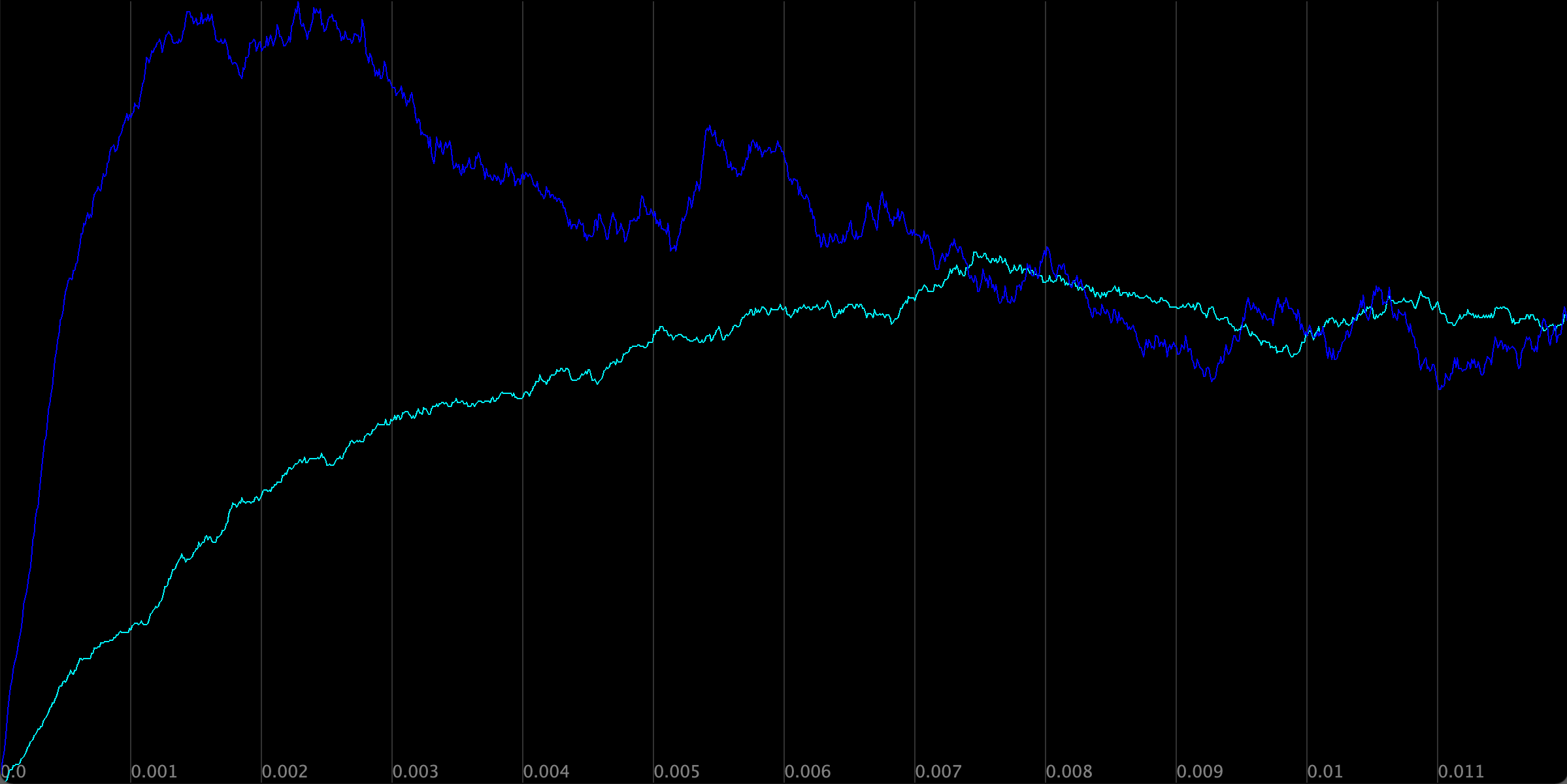 The concentration of Z in the two simulations. Simple activation of Z by X is shown in blue, and the type-1 incoherent FFL is shown in purple.
Note the different pattern to the growth of Z than we saw under negative autoregulation. When modeling negative autoregulation, the concentration of the protein approached steady state from below. In the case of the FFL, the concentration of Z grows so quickly that it passes its eventual steady state concentration and then returns to this steady state from above.
We can interpret from the model why the FFL allows for a fast response time as well as why it initially passes the steady state concentration. At the start of the simulation, Z is activated by X very quickly. X activates Y as well, but at a lower rate than the regulation of Z because Y only has its own degradation to slow this process. Therefore, more Z is initially produced than Y, which causes the concentration of Z to shoot past its eventual steady state.
The figure above is reminiscent of a damped oscillation process like the one in the figure below, in which the concentration of a particle oscillates above and below a steady state, while the amplitude of the wave gets smaller and smaller. We wonder: is it possible for a network motif to produce more of a true “wave” without dampening?
 In a damped oscillation, the value of some variable (shown on the y-axis) oscillates back and forth around an asymptotic value while the amplitude decreases over time (shown on the x-axis).3
-
Gene ontology database with “transcription” keyword: https://www.uniprot.org/. ↩
-
Mangan, S., & Alon, U. (2003). Structure and function of the feed-forward loop network motif. Proceedings of the National Academy of Sciences of the United States of America, 100(21), 11980–11985. https://doi.org/10.1073/pnas.2133841100 ↩
-
https://www.toppr.com/guides/physics/oscillations/damped-simple-harmonic-motion/ ↩
