Network Motifs Exercises

A short introduction to statistical validation

In this chapter, we have largely appealed to intuition when claiming that the number of network structures that we observe is larger than what we would see due to random chance. For example, we pointed out that there are 130 loops in the E. coli transcription factor network, but we would only expect to see 2.42 such loops if the network were random.

This argument hints at a foundational approach in statistics, which is to determine the likelihood that an observation would occur due to random chance; this likelihood is called a p-value. In this case, our observation is 130 loops, and the probability that this number of loops would have arisen in a random network of the same size is practically zero. The exact computation of this p-value is beyond the scope of our work here, but we will turn our attention to a different p-value that is easier to determine.

We also mentioned that 95 of the 130 loops in the E. coli transcription factor network correspond to repression, which is another surprising fact, since in a random network, we would expect to see only about 65 loops that correspond to activation. We therefore hypothesize that negative autoregulation is on the whole more important to the cell than positive autoregulation.

To compute a p-value associated with the frequency of negative autoregulation, we ask, “if the choice of a loop corresponding to activation or repession were random and equal, then what is the likelihood that out of 130 loops, 95 (or more) correspond to activation?” This question is biological but is equivalent to a question about flipping coins: “if we flip a coin 130 times, then what is the likelihood that the coin will come up heads 95 or more times?”

Say that we observe four coin flips. Then there are 16 equally likely outcomes, shown in the table below.

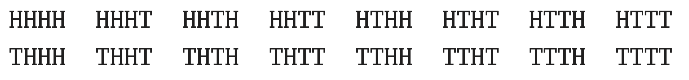The 16 possible sequences resulting from flipping a coin four times.

Each outcome is equally likely, and so we can compute the probability of observing k heads in the four flips by counting how many of the 16 cases have k heads:

\[\begin{align*} \mathrm{Pr}(\text{0 heads}) &= 1/16\,;\\ \mathrm{Pr}(\text{1 heads}) & = 4/16 = 1/4\,;\\ \mathrm{Pr}(\text{2 heads}) & = 6/16 = 3/8\,;\\ \mathrm{Pr}(\text{3 heads}) & = 4/16 = 1/4\,;\\ \mathrm{Pr}(\text{4 heads}) & = 1/16\,. \end{align*}\]

To generalize these probabilities, if we flip a coin n times, then the probability of obtaining k heads is equal to

\[\dbinom{n}{k} \cdot \left(\dfrac{1}{2}\right)^n\]

where \(\binom{n}{k}\) is called the “combination statistic” and is equal to n!/(k! · (n − k)!).

If we instead wish to compute the probability of obtaining at least k heads, then we simply need to sum the above expression for all values larger than k:

\[\displaystyle\sum\limits_{j=k}^n{\dbinom{n}{j} \cdot \left(\dfrac{1}{2}\right)^n}\]

This expression gives us our desired p-value.

Exercise: When n = 130 and k = 95, compute the p-value given by the above expression. Is it likely that random chance could have produced 95 out of 130 loops in the transcription factor network that correspond to repression?

Counting feedforward loops

Exercise: Modify the Jupyter notebook provided in the tutorial on loops to count the number of feed-forward loops in the transcription factor network for E. coli.

There are eight types of feed-forward loops based on the eight different ways in which we can label the edges in the network with a “+” or a “-“ based on activation or repression.

The eight types of feed-forward loops.¹

Exercise: Modify the Jupyter notebook to count the number of loops of each type in the E. coli transcription factor network.

Exercise: How many feed-forward loops would you expect to see in a random network having the same number of nodes as the E. coli transcription factor network? How does this compare to your answers to the previous two questions?

Negative autoregulation

Exercise: One way for the cell to apply stronger “brakes” to the activation of a transcription factor would be to simply increase the degradation rate of that transcription factor, rather than implement negative autoregulation. From an evolutionary perspective, why do you think that the cell doesn’t do this?

Recall that we used the reaction reaction X → X + Y to represent activation. We then built a model in a tutorial to run a mathematically controlled comparison between two simulated cells, one having only this reaction, and the other also having negative autoregulation, which we represented using the reaction Y + Y → Y.

Exercise: Multiply the rate of the reaction X → X + Y by a factor of 100 in the cell having only simple regulation, and plot the concentration of Y in both cells (the updated table containing reactants, products, and reaction rate constants is found below). By approximately what factor do you need to increase the rate of this reaction in the cell that includes negative autoregulation so that the steady-state concentration of Y remains the same in both cells?

Reactants	Products	Forward Rate
X1’	X1’ + Y1’	4e4
X2’	X2’ + Y2’	4e2
Y1’	NULL	4e2
Y2’	NULL	4e2
Y2’ + Y2’	Y2’	4e2

Positive autoregulation

Although most of the autoregulating E. coli transcription factors exhibit negative autoregulation, 35 of these transcription factors autoregulate positively, meaning that the transcription factor activates its own regulation. This network motif exists in processes in which the cell needs a cell to be produced at a slower, more precise rate than it would under normal activation. This occurs in some genes related to development, when gene expression must be carefully controlled.

Exercise: Design and implement a reaction-diffusion model to run a mathematically-controlled simulation comparing the positive autoregulation of a transcription factor Y against normal activation of Y by another transcription factor X. Plot the concentration of Y over time in the two simulations.

Replicating the module’s conclusions with well-mixed simulations

Recall that a repressilator is a network motif in which X inhibits Y, which inhibits Z, which in turn inhibits Z. In a tutorial, we showed how to use a well-mixed simulation to build the repressilator, which we then perturbed.\tutorial[motifs/tutorial_perturb]\

Exercise: Build well-mixed simulations to replicate the other network motif tutorials presented in this module.

Next module

1. Image adapted from Mangan, S., & Alon, U. (2003). Structure and function of the feed-forward loop network motif. Proceedings of the National Academy of Sciences of the United States of America, 100(21), 11980–11985. https://doi.org/10.1073/pnas.2133841100 ↩