 Leanpub
Oscillators are everywhere in nature
Even if placed in a windowless bunker without clocks, humans will maintain a roughly 24-hour cycle of sleep and wakefulness1. This circadian rhythm is present throughout many living things, including plants and even cyanobacteria2. Your heart and respiratory system also follow subconscious cyclical rhythms, and your cells are governed by a strict cell cycle as they grow and divide.
We might guess from what we have learned in this module that cyclical biological rhythms must be governed by simple rules. However, the question remains as to what these rules are and how they can correctly execute oscillations over and over.
Researchers have identified many network motifs that facilitate oscillation, some of which are very complicated and include many components. In this lesson, we will focus on a simple three-component oscillator motif.
The repressilator: a synthetic biological oscillator
The repressilator motif3 is shown in the figure below. In this motif, all three proteins are transcription factors, and they form a cycle in which X represses Y, Y represses Z, and Z represses X. The repressilator forms a feedback loop, but nothing a priori about this motif indicates that it would lead to oscillation.
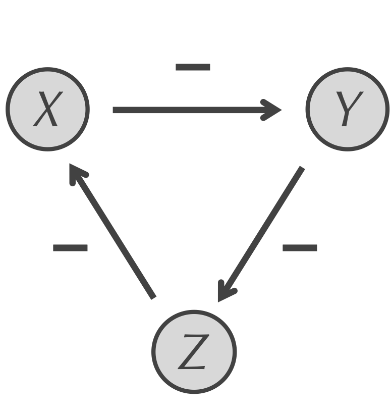 The repressilator motif for three particles X, Y, and Z. X represses Y, which represses Z, which in turn represses X, forming a feedback loop.
STOP: Devise a reaction-diffusion model representing the repressilator.
To build a reaction-diffusion model accompanying the repressilator, we start with a quantity of X particles and no Y or Z particles. We assume that all three particles diffuse at the same rate and degrade at the same rate.
Furthermore, we assume that all three particles are produced as the result of an activation process by some other transcription factor(s), which we assume happens at the same rate. We will use a single hidden particle I that serves to activate the three visible particles via the three reactions I → I + X, I → I + Y, and I → I + Z, all taking place at the same rate.
In the previous lesson on the feed-forward loop, we saw that we can use the reaction X + Y → X to model the repression of Y by X. To complete the repressilator model, we will supplement this reaction with the reactions Y + Z → Y and Z + X → Z, with all three repression reactions occurring at the same rate.
Note: To better reflect the biological reality of proteins regulating genes, we will need to add a few additional particles to our model differentiating transcription factor genes from the proteins that they encode. We leave the details to the tutorial below.
Interpreting the repressilator’s oscillations
The figure below plots the concentration over time of X, Y, and Z particles from our repressilator simulation (colored yellow, red, and blue, respectively). The system exhibits clear oscillatory behavior, with X, Y, and Z taking turns being at high concentration.
STOP: Why do you think that the repressilator motif leads to a pattern of oscillations?
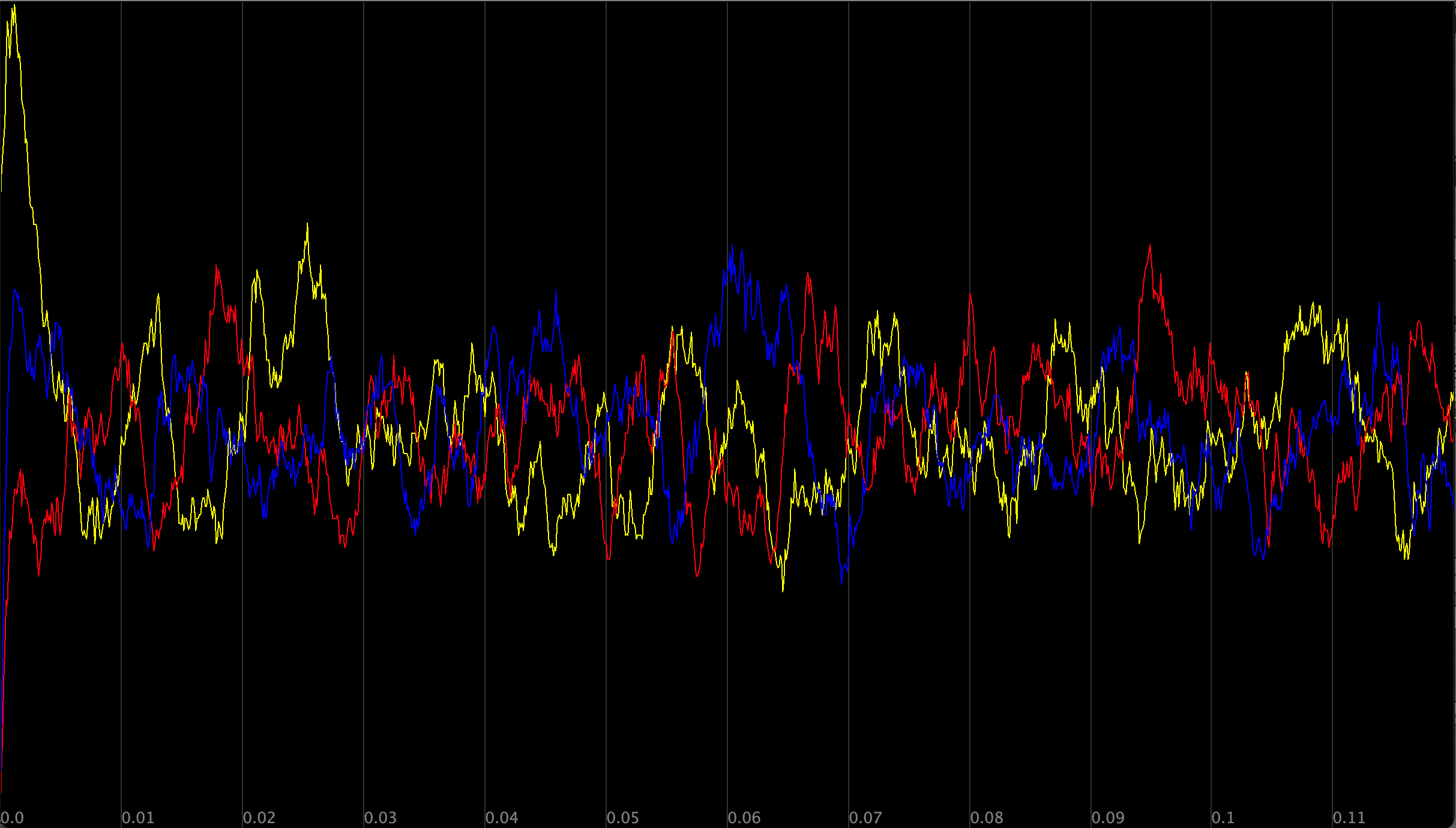 Modeling the repressilator’s concentration of each particle over time; X is shown in yellow, Y is shown in red, and Z is shown in blue.
Because the concentration of X starts out high, with no Y or Z present, the concentration of X briefly increases because its rate of production exceeds its rate of degradation. With no Y or Z particles present, there are none to degrade or be repressed, and so the concentrations of these particles start increasing as well. However, because X particles begin at high concentration, the repression reaction X + Y → X prevents the concentration of Y from growing as fast as the concentration of Z.
As the concentration of Z rises, the repression reaction Z + X → Z occurs often enough for the rate of removal of X to equal and exceed its rate of production, accounting for the first (yellow) peak in the figure above. The concentration of X then plummets, with the concentration of Z rising up to replace it. This situation is shown by the second (blue) peak in the figure above.
As a result, Z and X have switched roles. Because the concentration of Z is high and the concentration of Y is increasing, the reaction Y + Z → Y will occur frequently and reduce the concentration of Z. Furthermore, because the concentration of X has decreased and the concentration of Y is still relatively low, the reaction X + Y → X will occur less often, allowing the concentration of Y to continue to rise. Eventually, the decrease in the concentration of Z and the increase in the concentration of Y will account for the third (red) peak in the figure above.
At this point, the reaction X + Y → X will suppress the concentration of Y. Because the concentration of X and Z are both lower than the concentration of Z, the reaction Z + X → Z will not greatly influence the concentration of X, which will rise to meet the falling concentration of Y, and we have returned to our original situation, at which point the cycle will begin again.
Noise is a feature, not a bug
Take another look at the figure showing the oscillations of the repressilator. You will notice that the concentrations zigzag as they travel up or down, and that they peak at slightly different levels each time.
This noise in the repressilator’s oscillations is due to random variation as the particles bounce around due to diffusion. The repression reactions require two particles to collide, and these collisions may occur more or less often than expected because of random chance, which is exacerbated by low sample size. We have around 150 molecules at each peak in the above figure, but a given cell may have 1,000 to 10,000 molecules of a single protein.4
Yet the noise in the repressilator’s oscillations is a feature, not a bug. As we have discussed previously, the cell’s molecular interactions are inherently random. If we see oscillations in a simulation built on randomness, then we can be confident that this simulation is robust to a certain amount of variation.
In this module’s conclusion, we will further explore the concept of robustness as it pertains to the repressilator. What happens if our simulation experiences a much greater disturbance to the concentration of one of the particles? Will it still be able to recover and return to the same oscillatory pattern?
-
Aschoff, J. (1965). Circadian rhythms in man. Science 148, 1427–1432. ↩
-
Grobbelaar N, Huang TC, Lin HY, Chow TJ. 1986. Dinitrogen-fixing endogenous rhythm in Synechococcus RF-1. FEMS Microbiol Lett 37:173–177. doi:10.1111/j.1574-6968.1986.tb01788.x.CrossRefWeb of Science. ↩
-
Elowitz MB, Leibler S. A synthetic oscillatory network of transcriptional regulators. Nature. 2000;403(6767):335-338. doi:10.1038/35002125 ↩
-
Brandon Ho, Anastasia Baryshnikova, Grant W. Brown. Unification of Protein Abundance Datasets Yields a Quantitative Saccharomyces cerevisiae Proteome. Cell Systems, 2018; DOI: 10.1016/j.cels.2017.12.004 ↩
