Software Tutorial: Traveling Down an Attractant Gradient

In the previous tutorial, we simulated the behavior of a bacterium moving up the concentration gradient. In this tutorial, we will simulate the opposite - when the bacterium is not in luck and moves down a concentration gradient.

To get started, open Visual Studio Code, and click File > Open Folder.... Open the EColiSimulations folder from the first tutorial. If you would rather not follow along below, you can download a completed BioNetGen file here: removal.bngl.

We also will build a Jupyter notebook in this tutorial for plotting the concentrations of different particles over time. To do so, you should save a copy of your plotter_up.ipynb file called plotter_down.ipynb; if you would rather not follow along, we provide a completed notebook here: plotter_down.ipynb

Before running this notebook, make sure the following dependencies are installed.

Installation Link	Version	Check install/version
Python3	3.6+	python --version
Jupyter Notebook	4.4.0+	jupyter --version
Numpy	1.14.5+	pip list \| grep numpy
Matplotlib	3.0+	pip list \| grep matplotlib
Colorspace or with pip	any	pip list \| grep colorspace

Modeling a decreasing ligand gradient with a BioNetGen function

We have simulated how the concentration of phosphorylated CheY changes when the cell moves up the attractant gradient. The concentration dips, but over time, methylation states change so that they can compensate for the increased ligand-receptor binding and restore the equilibrium of phosphorylated CheY. What if instead ligands are removed, as we would see if the bacterium is traveling down an attractant gradient? We might imagine that we would see an increase in phosphorylated CheY to increase tumbling and change course, followed by a return to steady state. But is this what we will see?

To simulate the cell traveling down an attractant gradient, we will add a kill reaction removing unbound ligand at a constant rate. To do so, we will add the following rule within the reaction rules section.

#Simulate ligand removal
LigandGone: L(t) -> 0 k_gone

In the parameters section, we start by defining k_gone to be 0.3, so that d[L]/dt = -0.3[L]. The solution of this differential equation is [L] = 10⁷e^-0.3t. We will also change the initial ligand concentration (L0) to be 1e7. Thus, the concentration of ligand becomes so low that ligand-receptor binding reaches 0 within 50 seconds.

k_gone 0.3
L0 1e7

We will set the initial concentrations of all species to be the final steady state concentrations from the result for our adaptation.bngl model, and see if after reducing the concentration of unbound ligand gradually, the simulation can restore these concentrations to steady state.

First, visit the adaptation.bngl model and add the concentration for each combination of methylation state and ligand binding state of the receptor complex to the observables section. Then run this simulation with L0 equal to 1e7.

When the simulation is finished, visit the adaptation folder from the adaptation tutorial and find the simulation result at the final time point.

When the model finishes running, input the final concentrations of molecules to the species section of our removal.bngl model. Here is what we have.

begin species
	@EC:L(t) L0
	@PM:T(l!1,r,Meth~A,Phos~U).L(t!1) 1190
	@PM:T(l!1,r,Meth~B,Phos~U).L(t!1) 2304
	@PM:T(l!1,r,Meth~C,Phos~U).L(t!1) 2946
	@PM:T(l!1,r,Meth~A,Phos~P).L(t!1) 2
	@PM:T(l!1,r,Meth~B,Phos~P).L(t!1) 156
	@PM:T(l!1,r,Meth~C,Phos~P).L(t!1) 402
	@CP:CheY(Phos~U) CheY0*0.71
	@CP:CheY(Phos~P) CheY0*0.29
	@CP:CheZ() CheZ0
	@CP:CheB(Phos~U) CheB0*0.62
	@CP:CheB(Phos~P) CheB0*0.38
	@CP:CheR(t) CheR0
end species

Running the BioNetGen model

We are now ready to run our BioNetGen model. To do so, first add the following after end model to run our simulation over 1800 seconds.

generate_network({overwrite=>1})
simulate({method=>"ssa", t_end=>1800, n_steps=>1800})

The following code contains our complete simulation, which can also be downloaded here: removal.bngl.

begin model

begin molecule types
	L(t)
	T(l,r,Meth~A~B~C,Phos~U~P)
	CheY(Phos~U~P)
	CheZ()
	CheB(Phos~U~P)
	CheR(t)
end molecule types

begin observables
	Molecules bound_ligand L(t!1).T(l!1)
	Molecules phosphorylated_CheY CheY(Phos~P)
	Molecules low_methyl_receptor T(Meth~A)
	Molecules medium_methyl_receptor T(Meth~B)
	Molecules high_methyl_receptor T(Meth~C)
	Molecules phosphorylated_CheB CheB(Phos~P)
end observables

begin parameters
	NaV2 6.02e8   #Unit conversion to cellular concentration M/L -> #/um^3
	miu 1e-6

	L0 1e7
	T0 7000
	CheY0 20000
	CheZ0 6000
	CheR0 120
	CheB0 250

	k_lr_bind 8.8e6/NaV2  #ligand-receptor binding
	k_lr_dis 35            #ligand-receptor dissociation

	k_TaUnbound_phos 7.5   #receptor complex autophosphorylation

	k_Y_phos 3.8e6/NaV2   #receptor complex phosphorylates Y
	k_Y_dephos 8.6e5/NaV2  #Z dephosphorylates Y

	k_TR_bind  2e7/NaV2 #Receptor-CheR binding
	k_TR_dis   1          #Receptor-CheR dissociation
	k_TaR_meth 0.08       #CheR methylates receptor complex

	k_B_phos 1e5/NaV2      #CheB phosphorylation by receptor complex
	k_B_dephos 0.17       #CheB autodephosphorylation

	k_Tb_demeth 5e4/NaV2   #CheB demethylates receptor complex
	k_Tc_demeth 2e4/NaV2 #CheB demethylates receptor complex

	k_gone 0.3
end parameters

begin reaction rules
	LigandReceptor: L(t) + T(l) <-> L(t!1).T(l!1) k_lr_bind, k_lr_dis

	#Receptor complex (specifically CheA) autophosphorylation
	#Rate dependent on methylation and binding states
	#Also on free vs. bound with ligand
	TaUnboundP: T(l,Meth~A,Phos~U) -> T(l,Meth~A,Phos~P) k_TaUnbound_phos
	TbUnboundP: T(l,Meth~B,Phos~U) -> T(l,Meth~B,Phos~P) k_TaUnbound_phos*1.1
	TcUnboundP: T(l,Meth~C,Phos~U) -> T(l,Meth~C,Phos~P) k_TaUnbound_phos*2.8
	TaLigandP: L(t!1).T(l!1,Meth~A,Phos~U) -> L(t!1).T(l!1,Meth~A,Phos~P) 0
	TbLigandP: L(t!1).T(l!1,Meth~B,Phos~U) -> L(t!1).T(l!1,Meth~B,Phos~P) k_TaUnbound_phos*0.8
	TcLigandP: L(t!1).T(l!1,Meth~C,Phos~U) -> L(t!1).T(l!1,Meth~C,Phos~P) k_TaUnbound_phos*1.6

	#CheY phosphorylation by T and dephosphorylation by CheZ
	YPhos: T(Phos~P) + CheY(Phos~U) -> T(Phos~U) + CheY(Phos~P) k_Y_phos
	YDephos: CheZ() + CheY(Phos~P) -> CheZ() + CheY(Phos~U) k_Y_dephos

	#CheR binds to and methylates receptor complex
	#Rate dependent on methylation states and ligand binding
	TRBind: T(r) + CheR(t) <-> T(r!2).CheR(t!2) k_TR_bind, k_TR_dis
	TaRUnboundMeth: T(r!2,l,Meth~A).CheR(t!2) -> T(r,l,Meth~B) + CheR(t) k_TaR_meth
	TbRUnboundMeth: T(r!2,l,Meth~B).CheR(t!2) -> T(r,l,Meth~C) + CheR(t) k_TaR_meth*0.1
	TaRLigandMeth: T(r!2,l!1,Meth~A).L(t!1).CheR(t!2) -> T(r,l!1,Meth~B).L(t!1) + CheR(t) k_TaR_meth*30
	TbRLigandMeth: T(r!2,l!1,Meth~B).L(t!1).CheR(t!2) -> T(r,l!1,Meth~C).L(t!1) + CheR(t) k_TaR_meth*3

	#CheB is phosphorylated by receptor complex, and autodephosphorylates
	CheBphos: T(Phos~P) + CheB(Phos~U) -> T(Phos~U) + CheB(Phos~P) k_B_phos
	CheBdephos: CheB(Phos~P) -> CheB(Phos~U) k_B_dephos

	#CheB demethylates receptor complex
	#Rate dependent on methyaltion states
	TbDemeth: T(Meth~B) + CheB(Phos~P) -> T(Meth~A) + CheB(Phos~P) k_Tb_demeth
	TcDemeth: T(Meth~C) + CheB(Phos~P) -> T(Meth~B) + CheB(Phos~P) k_Tc_demeth

	#Simulate ligand removal
	LigandGone: L(t) -> 0 k_gone

end reaction rules

begin compartments
  EC  3  100       #um^3
  PM  2  1   EC    #um^2
  CP  3  1   PM    #um^3
end compartments

begin species
	@EC:L(t) L0
	@PM:T(l!1,r,Meth~A,Phos~U).L(t!1) 1190
	@PM:T(l!1,r,Meth~B,Phos~U).L(t!1) 2304
	@PM:T(l!1,r,Meth~C,Phos~U).L(t!1) 2946
	@PM:T(l!1,r,Meth~A,Phos~P).L(t!1) 2
	@PM:T(l!1,r,Meth~B,Phos~P).L(t!1) 156
	@PM:T(l!1,r,Meth~C,Phos~P).L(t!1) 402
	@CP:CheY(Phos~U) CheY0*0.71
	@CP:CheY(Phos~P) CheY0*0.29
	@CP:CheZ() CheZ0
	@CP:CheB(Phos~U) CheB0*0.62
	@CP:CheB(Phos~P) CheB0*0.38
	@CP:CheR(t) CheR0
end species

end model

generate_network({overwrite=>1})
simulate({method=>"ssa", t_end=>1800, n_steps=>1800})

Now save your file and run the simulation by clicking Run BNG. The results will be saved in a new folder called removal/TIME contained in the current directory. Rename the folder from the timestamp to the value of k_gone, 0.3.

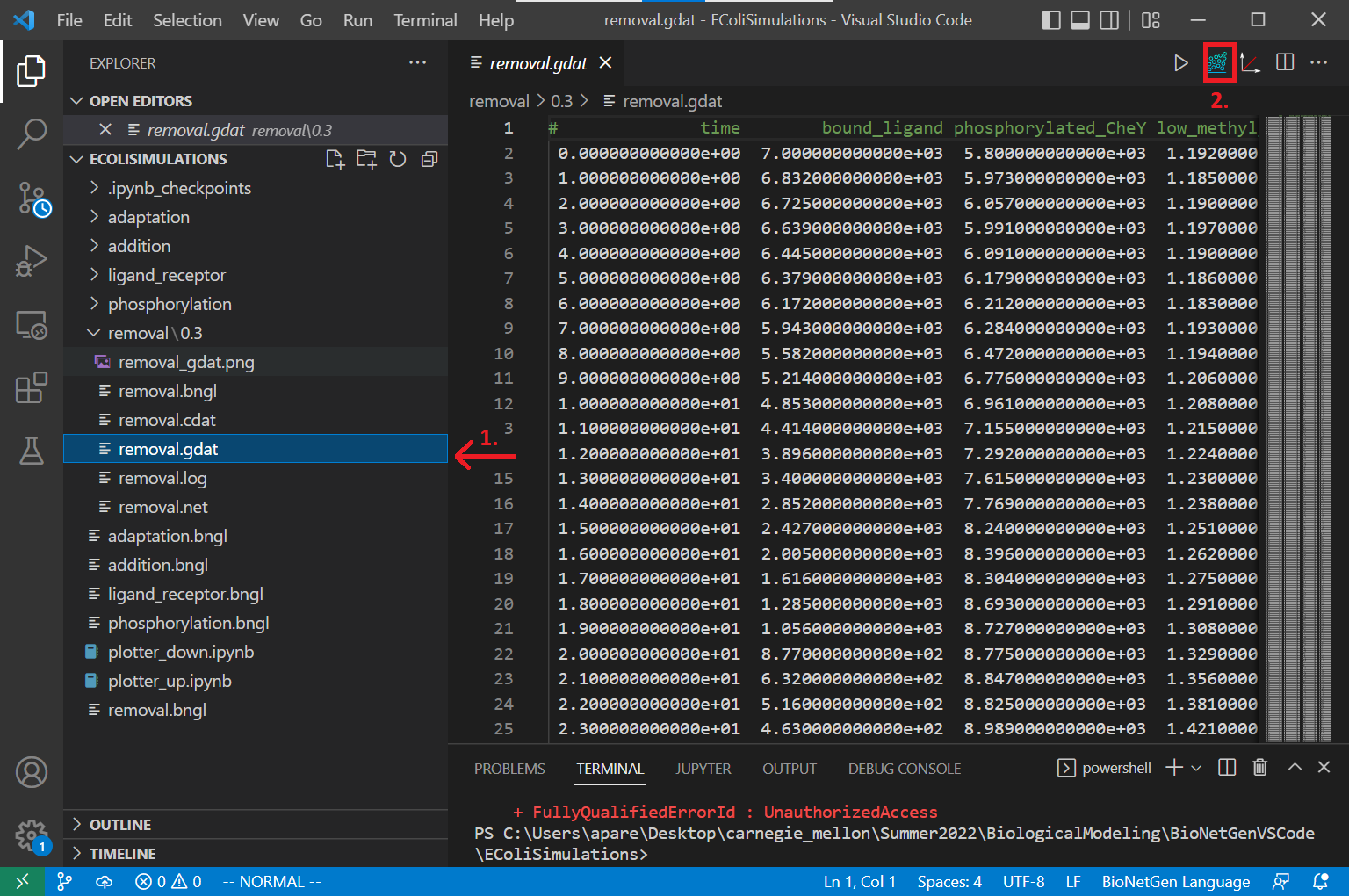
Open the newly created removal.gdat file and create a plot by clicking the Built-in plotting button.

What happens to the concentration of phosphorylated CheY? Are the concentrations of complexes at different methylation states restored to their levels before adding ligands to the adaptation.bngl model?

As we did in the tutorial simulating increasing ligand, we can try different values for k_gone. Change t_end in the simulate method to 1800 seconds, and run the simulation with k_gone equal to 0.01, 0.03, 0.05, 0.1, and 0.5.

Note: All simulation results are stored in the removal directory in your working directory. As you change the values of k_gone, rename the directory with the k_gone values instead of the timestamp for simplicity.

Visualizing the results of our simulation

We will use the jupyter notebook plotter_up.ipynb as a template for the plotter_down.ipynb file that we will use to visualize our results. First, we will specify the directories, model name, species of interest, and reaction rates. Put the Jupyter notebook in the same directory as removal.bngl or change the model_path accordingly.

model_path = "removal"  #The folder containing the model
model_name = "removal"  #Name of the model
target = "phosphorylated_CheY"    #Target molecule
vals = [0.01, 0.03, 0.05, 0.1, 0.3, 0.5]  #Gradients of interest

The second code block is the same as that provided in the previous tutorial. This code loads the simulation result at each time point from the .gdat file, which stores the concentration of all observables at all steps. It then plots the concentration of phosphorylated CheY over time.

import numpy as np
import sys
import os
import matplotlib.pyplot as plt
import colorspace


#Define the colors to use
colors = colorspace.qualitative_hcl(h=[0, 300.], c = 60, l = 70, pallete = "dynamic")(len(vals))


def load_data(val):
    file_path = os.path.join(model_path, str(val), model_name + ".gdat")
    with open(file_path) as f:
        first_line = f.readline() #Read the first line
    cols = first_line.split()[1:] #Get the col names (species names)

    ind = 0
    while cols[ind] != target:
        ind += 1                  #Get col number of target molecule

    data = np.loadtxt(file_path)  #Load the file
    time = data[:, 0]             #Time points
    concentration = data[:, ind]  #Concentrations

    return time, concentration


def plot(val, time, concentration, ax, i):
    legend = "k = - " + str(val)
    ax.plot(time, concentration, label = legend, color = colors[i])
    ax.legend()

    return


fig, ax = plt.subplots(1, 1, figsize = (10, 8))
for i in range(len(vals)):
    val = vals[i]
    time, concentration = load_data(val)
    plot(val, time, concentration, ax, i)

plt.xlabel("time")
plt.ylabel("concentration (#molecules)")
plt.title("Active CheY vs time")
ax.minorticks_on()
ax.grid(b = True, which = 'minor', axis = 'both', color = 'lightgrey', linewidth = 0.5, linestyle = ':')
ax.grid(b = True, which = 'major', axis = 'both', color = 'grey', linewidth = 0.8 , linestyle = ':')

plt.show()

Run the notebook. How does the value of k_gone impact the concentration of phosphorylated CheY? Why? Are the tumbling frequencies restored to the background frequency? As we return to the main text, we will show the resulting plots and discuss these questions.

Return to main text