Stochastic Simulation of Chemical Reactions

Verifying a theoretical steady state concentration via stochastic simulation

In the previous module, we saw that we could avoid tracking the positions of individual particles if we assume that the particles are well-mixed, i.e., uniformly distributed throughout their environment. We will apply this assumption in our current work as well, in part because the E. coli cell is so small. As a proof of concept, we will see if a well-mixed simulation replicates a reversible reaction’s equilibrium concentrations of particles that we found in the previous lesson.

Even though we can calculate steady state concentrations manually, a particle-free simulation will be useful for two reasons. First, this simulation will give us snapshots of the concentrations of particles in the system over multiple time points and allow us to see how quickly the concentrations reach equilibrium. Second, we will soon expand our model of chemotaxis to have many particles and reactions that depend on each other, and direct mathematical analysis of the system will become impossible.

Note: The difficulty posed to precise analysis of systems with multiple chemical reactions is comparable to the famed “n-body problem” in physics. Predicting the motions of two celestial objects interacting due to gravity can be done exactly, but once we add more bodies to the system, no exact solution exists, and we must rely on simulation.

Our particle-free model will apply an approach called Gillespie’s stochastic simulation algorithm, which is often called the Gillespie algorithm or just SSA for short. Before we explain how this algorithm works, we will take a short detour to provide some needed probabilistic context.

The Poisson and exponential distributions

Imagine that you own a store and have noticed that on average, λ customers enter your store in a single hour. Let X denote the number of customers entering the store in the next hour; X is an example of a random variable because its value may change depending on random chance. If we assume that customers are independent actors, then X follows a Poisson distribution. It can be shown that for a Poisson distribution, the probability that exactly n customers arrive in the next hour is

\[\mathrm{Pr}(X = n) = \dfrac{\lambda^n e^{-\lambda}}{n!}\,,\]

where e is the mathematical constant known as Euler’s number and is equal to 2.7182818284…

Note: A derivation of the above formula for Pr(X = n) is beyond the scope of our work here, but if you are interested in one, please check out this article by Andrew Chamberlain.

Furthermore, the probability of observing exactly n customers in t hours, where t is an arbitrary positive number, is

\[\dfrac{(\lambda t)^n e^{-\lambda t}}{n!}\,.\]

We can also ask how long we will typically have to wait for the next customer to arrive. Specifically, what are the chances that this customer will arrive after t hours? If we let T be the random variable corresponding to the wait time on the next customer, then the probability of T being at least t is the probability of seeing zero customers in t hours:

\[\mathrm{Pr}(T > t) = \mathrm{Pr}(X = 0) = \dfrac{(\lambda t)^0 e^{-\lambda t}}{0!} = e^{-\lambda t}\,.\]

In other words, the probability Pr(T > t) that the wait time is longer than time t decays exponentially as t increases. For this reason, the random variable T is said to follow an exponential distribution. It can be shown that the expected value of the exponential distribution (i.e., the average amount of time that we will need to wait for the next event to occur) is 1/λ.

STOP: What is the probability Pr(T < t)?

The Gillespie algorithm

We now return to explain the Gillespie algorithm for simulating multiple chemical reactions in a well-mixed environment. The engine of this algorithm runs on a single question: given a well-mixed environment of particles and a reaction involving those particles taking place at some average rate, how long should we expect to wait before this reaction occurs somewhere in the environment?

This is the same question that we asked in the previous discussion; we have simply replaced customers entering a store with instances of a chemical reaction. The average number λ of occurrences of the reaction in a unit time period is the rate r at which the reaction occurs. Therefore, an exponential distribution with average wait time 1/r can be used to model the time between instances of the reaction.

Next, say that we have two reactions proceeding independently of each other and occurring at rates r₁ and r₂. The combined average rates of the two reactions is r₁ + r₂, which is also a Poisson distribution. Therefore, the wait time required to wait for either of the two reactions is exponentially distributed, with an average wait time equal to 1/(r₁ + r₂).

Numerical methods allow us to generate a random number simulating the wait time of an exponential distribution. By repeatedly generating these numbers, we can obtain a series of wait times between consecutive reaction occurrences.

Once we have generated a wait time, we should determine the reaction to which it corresponds. If the rates of the two reactions are equal, then we simply choose one of the two reactions randomly with equal probability. But if the rates of these reactions are different, then we should choose one of the reactions via a probability that is weighted in direct proportion to the rate of the reaction; that is, the larger the rate of the reaction, the more likely that this reaction corresponds to the current event.¹ To do so, we select the first reaction with probability r₁/(λ₁ + r₂) and the second reaction with probability r₂/(r₁ + r₂). (Note that these two probabilities sum to 1.)

As illustrated in the figure below, we will demonstrate the Gillespie algorithm by returning to our ongoing example, in which we are modeling the forward and reverse reactions of ligand-receptor binding and dissociation. These reactions have rates r_bind = k_bind · [L] · [T] and r_dissociate = k_dissociate · [LT], respectively.

First, we choose a wait time according to an exponential distribution with mean value 1/(r_bind + r_dissociate). Then, the probability that the event corresponds to a binding reaction is given by

Pr(L + T → LT) = r_bind/(r_bind + r_dissociate),

and the probability that it corresponds to a dissociation reaction is

Pr(LT → L + T) = r_dissociate/(r_bind + r_dissociate).

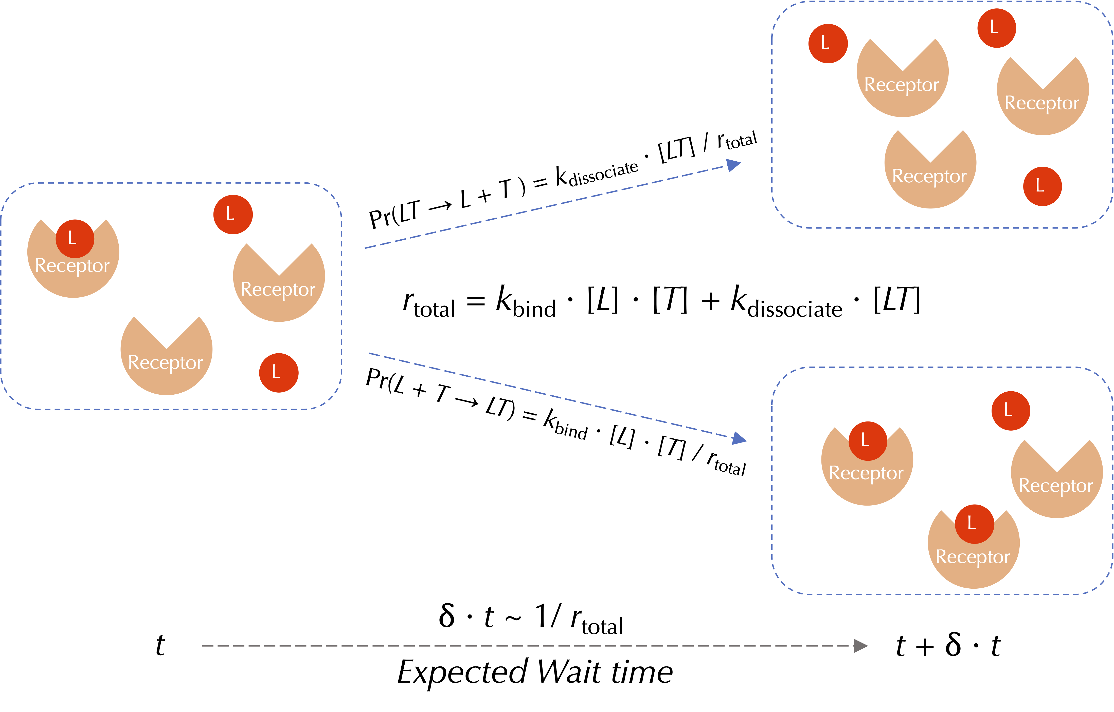A visualization of a single reaction event used by the Gillespie algorithm for ligand-receptor binding and dissociation. Red circles represent ligands (L), and orange wedges represent receptors (T). The wait time for the next reaction is drawn from an exponential distribution with mean 1/(k_bind + k_dissociate). The probability of this event corresponding to a binding or dissociation reaction is proportional to the rate of the respective reaction.

To generalize the Gillespie algorithm to n reactions occurring at rates r₁, r₂, …, r_n, the wait time between reactions will be exponentially distributed with average 1/(r₁ + r₂ + … + r_n). Once we select the next reaction to occur, the likelihood that it is the i-th reaction is equal to

r_i /(r₁ + r₂ + … + r_n).

Throughout this module, we will employ BioNetGen to apply the Gillespie algorithm to well-mixed models of chemical reactions. We will use our ongoing example of ligand-receptor binding and dissociation to introduce the way in which BioNetGen represents molecules and reactions involving them. The following tutorial shows how to implement this rule in BioNetGen and use the Gillespie algorithm to determine the equilibrium of a reversible ligand-receptor binding reaction.

Visit tutorial

Does the Gillespie algorithm confirm our steady state calculations?

In the previous lesson, we showed an example in which a system with 10,000 free ligand molecules and 7,000 free receptor molecules produced the following steady state concentrations using the experimentally verified binding rate of k_bind = 0.0146((molecules/µm³)^-1)s^-1 and dissociation rate of k_dissociate = 35s^-1:

• [LT] = 4,793 molecules/µm³;
• [L] = 5,207 molecules/µm³;
• [T] = 2,207 molecules/µm³.

Our model uses the same number of initial molecules and the same reaction rates. The system evolves via the Gillespie algorithm, and we track the concentration of free ligand molecules, ligand molecules bound to receptor molecules, and free receptor molecules over time.

The figure below demonstrates that the Gillespie algorithm quickly converges quickly to the same values calculated just above. Furthermore, the system reaches steady state in a fraction of a second.

A concentration plot over time for ligand-receptor dynamics via a BioNetGen simulation employing the Gillespie algorithm. Time is shown (in seconds) on the x-axis, and concentration is shown (in molecules/µm³) on the y-axis. The molecules quickly reach steady state concentrations that match those identified by hand.

This simple ligand-receptor model is just the beginning of our study of chemotaxis. In the next section, we will delve into the complex biochemical details of chemotaxis. Furthermore, we will see that the Gillespie algorithm for stochastic simulations will scale easily as our model of this system grows more complex.

Next lesson

1. Schwartz R. Biological Modeling and Simulaton: A Survey of Practical Models, Algorithms, and Numerical Methods. Chapter 17.2. ↩