 Leanpub
Two randomized exploration strategies
In the prologue, we saw that a particle taking a collection of n unit steps in random directions will wind up on average a distance proportional to \(\sqrt{n}\) units away from its starting position. We now will compare such a random walk against a modified algorithm that emulates the behavior of E. coli by changing the length of a step (i.e., how long the bacterium tumbles) based on the relative change in background attractant concentration.
We will represent a bacterium as a particle traveling in two-dimensional space. Units of distance will be measured in µm; recall from the introduction that a bacterium can cover 20 µm in a second during an uninterrupted run. The bacterium will start at the origin (0, 0).
We will use L(x, y) to denote the ligand concentration at (x, y) and establish a point (called the goal) at which L(x, y) is maximized. We will place the goal at (1500, 1500), so that the bacterium must travel a significant distance from the origin to reach the goal.
We would like the ligand concentration L(x, y) to decrease exponentially the farther we travel from the goal. We therefore set L(x, y) = 100 · 106 · (1-d/D), where d is the distance from (x, y) to the goal, and D is the distance from the origin to the goal, which in this case is 1500√2 ≈ 2121 µm. At the origin, the attractant concentration is equal to 100, and at the goal, the attractant concentration is equal to 100,000,000.
STOP: How can we quantify how well a bacterium has done at finding the attractant?
We are comparing two different cellular behaviors, and so in the spirit of Module 1, we will simulate many random walks of a particle following each of the two strategies, described in what follows. (The total time needed by our simulation should be large enough to allow the bacterium to have enough time to reach the goal.) For each strategy, we will then measure how far on average a bacterium with each strategy is from the goal at the end of the simulation.
Strategy 1: Standard random walk
To model a particle following an “unintelligent” random walk strategy, we first select a random direction of movement along with a duration of tumble. The angle of reorientation is a random number selected uniformly between 0° and 360°. The duration of each tumble is a “wait time” of sorts and follows an exponential distribution with experimentally verified mean equal to 0.1 seconds1. As the result of a tumble, the cell only changes its orientation, not its position.
We then select a random duration to run and let the bacterium run in that direction for the specified amount of time. The duration of each run follows an exponential distribution with mean equal to the experimentally verified value of 1 second.
We then iterate the two steps of tumbling and running until the total time allocated for the simulation has elapsed.
In the following tutorial, we simulate this naive strategy using a Jupyter notebook that will also help us visualize the results of the simulation.
Strategy 2: Chemotactic random walk
In our second strategy, which we call the “chemotactic strategy”, we mimic the real response of E. coli to its environment based on what we have learned about chemotaxis throughout this module. The simulated bacterium will still follow a run and tumble model, but the duration of each run, which is a function of the bacterium’s tumbling frequency, will depend on the relative change in attractant concentration that it detects.
To ensure a mathematically controlled comparison, we will use the same approach for sampling the duration of a tumble and the direction of a run as in the first strategy.
We have seen in this module that it takes E. coli about half a second to respond to a change in attractant concentration. We use tresponse to denote this “response time”; to produce a reasonable model of chemotaxis, we will check the attractant concentration of a running particle at the particle’s current location every tresponse seconds.
We will then measure the percentage difference between the attractant concentration L(x, y) at the cell’s current point and the attractant concentration at the cell’s previous point, tresponse in the past; we denote this difference as Δ[L]. If Δ[L] is equal to zero, then the probability of a tumble in the next tresponse seconds should be the same as the likelihood of a tumble in the first strategy over the same time period. If Δ[L] is positive, then the probability of a tumble should be greater than it was in strategy 1; if Δ[L] is negative, then the probability of a tumble should be less than it was in strategy 1.
To model the relationship between the likelihood of a tumble and the value of Δ[L], we will let t0 denote the mean background run duration, which in the first strategy was equal to one second. We would like to use a simple formula for the expected run duration, such as t0 * (1 + 10 · Δ[L]).
Unfortunately, there are two issues with this formula. First, if Δ[L] is less than -0.1, then the run duration could be negative. Second, if Δ[L] is large, then the bacterium will run for so long that it could reach the goal and run past it.
To fix the first issue, we will first take the maximum of t0 * (1 + 10 · Δ[L]) and some small positive number c (we will use c equal to 0.000001). As for the second issue, we will then take the minimum of the resulting expression and 4 · t0. The final value,
μ = min(max(t0 * (1 + 10 · Δ[L]), c), 4 · t0),
becomes the mean run duration of a bacterium based on the recent relative change in concentration.
STOP: What is the mean run duration μ when Δ[L] is equal to zero? Is this what we would hope?
As with the first strategy, our simulated cell will alternate between tumbling and running in a random direction until the total time devoted to the simulation has elapsed. The only difference in the second strategy is that we will measure the percentage change in concentration Δ[L] between a cell’s current point and its previous point every tresponse seconds. After determining a mean run time μ according to the expression above, we will sample a random number p from an exponential distribution with mean μ, and the cell will tumble after p seconds if p is smaller than tresponse.
In the following tutorial, we will adapt the Jupyter notebook that we built in the previous tutorial to simulate this second strategy and run it many times, taking the average of the simulated bacteria’s distance to the goal.
Comparing the effectiveness of our two random walk strategies
The following figure visualizes the trajectories of three cells over 500 seconds using strategy 1 (left) and strategy 2 (right) with a default tumbling frequency t0 of one second. Unlike the cells following strategy 1, the cells following strategy 2 quickly hone in on the goal and remain near it.
 Three sample trajectories for the standard random walk strategy (left) and chemotactic random walk strategy (right). The standard random walk strategy is shown on the left, and the chemotactic random walk is shown on the right. Redder regions correspond to higher concentrations of ligand, with a goal having maximum concentration at the point (1500, 1500), which is indicated with a blue square. Each particle’s walk is colored from darker to lighter colors across the time frame of its trajectory.
We should be wary of such a small sample size. To confirm that what we observed in these trajectories is true in general, we will compare the two strategies over many simulations. The following figure visualizes the particle’s average distance to the goal over 500 simulations for both strategies and confirms our previous observation that strategy 2 is effective at guiding the simulated particle to the goal. And yet the direction of travel in this strategy is random, so why would this strategy be so successful?
 Distance to the goal plotted over time for 500 simulated particles following the standard random walk strategy (pink) and the chemotactic random walk strategy (green). The dark lines indicate the average distance over all simulations, and the shaded area around each line represents one standard deviation from the average.
The chemotactic strategy works because of a “rubber band” effect. If the bacterium is traveling down an attractant gradient (i.e., away from an attractant), then it is not allowed to travel very far in a single step before it is forced to tumble. If an increase of attractant is detected, however, then the cell can travel farther in a single direction before tumbling. On average, this effect serves to pull the bacterium in the direction of increasing attractant, even though the directions in which it travels are random.
A tiny change to a simple, unsuccessful randomized algorithm can therefore produce an elegant approach for exploring an unknown environment. But we left one more question unanswered: why is the default frequency of one tumble per second stable across a wide range of bacteria? To address this question, we will see how changing t0, the default time for a run step in the absence of change in attractant concentration, affects the ability of a simulated bacterium following strategy 2 to reach the goal. You may like to adjust the value of t0 in the previous tutorial yourself, or follow the tutorial below.
Why is background tumbling frequency constant across bacterial species?
The following figures show three trajectories for a few different values of t0 and a simulation that lasts for 800 seconds. First, we set t0 equal to 0.2 seconds and see that the simulated bacteria are not able to walk far enough in a single step to head toward the goal.
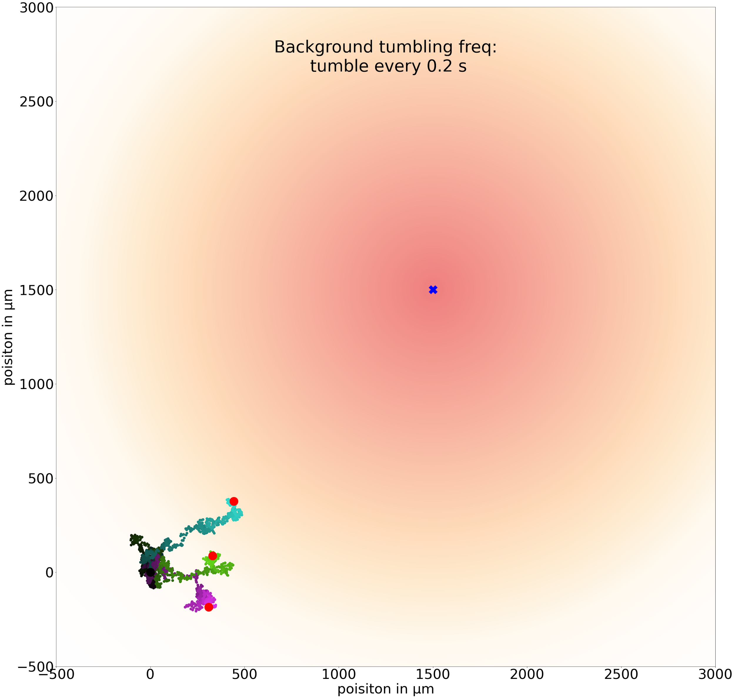 Three sample trajectories of a simulated cell following the chemotactic random walk strategy with an average run time between tumbles t0 of 0.2 seconds.
If we increase t0 to 5.0 seconds, then cells can run for so long that they may run past the goal without being able to brake by tumbling.
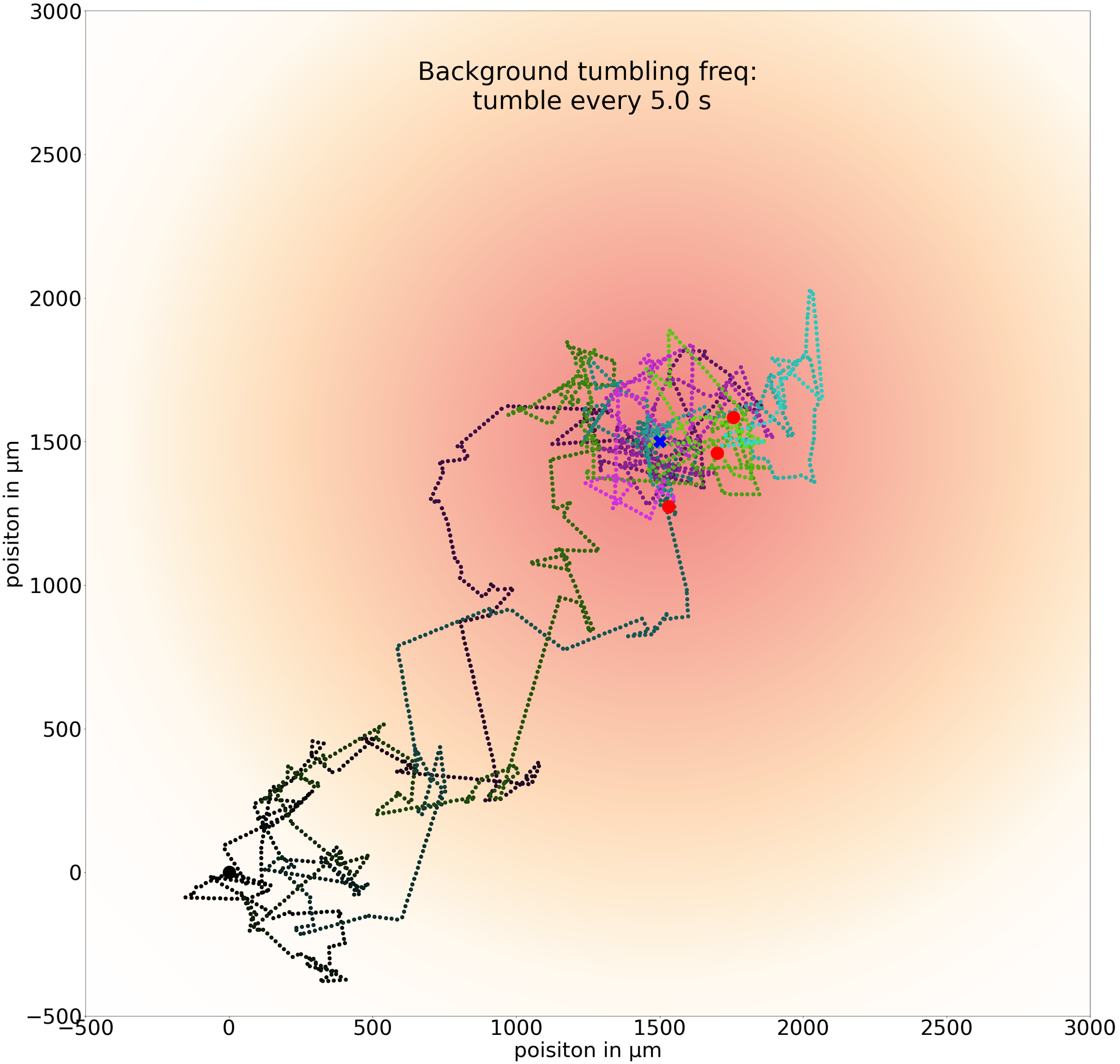 Three sample trajectories of a simulated cell following the chemotactic random walk strategy with an average run time between tumbles t0 of 5.0 seconds.
When we set t0 equal to 1.0, then the figure below shows a “Goldilocks” effect in which the simulated bacterium can run for long enough at a time to head quickly toward the goal, and it tumbles frequently enough to keep it near the goal.
 Three sample trajectories of a simulated cell following the chemotactic random walk strategy with an average run time between tumbles t0 of 1.0 seconds.
The figure below visualizes average particle distance to the goal over time for 500 particles using a variety of choices of t0. It confirms that tumbling every second by default is “just right” for finding an attractant.
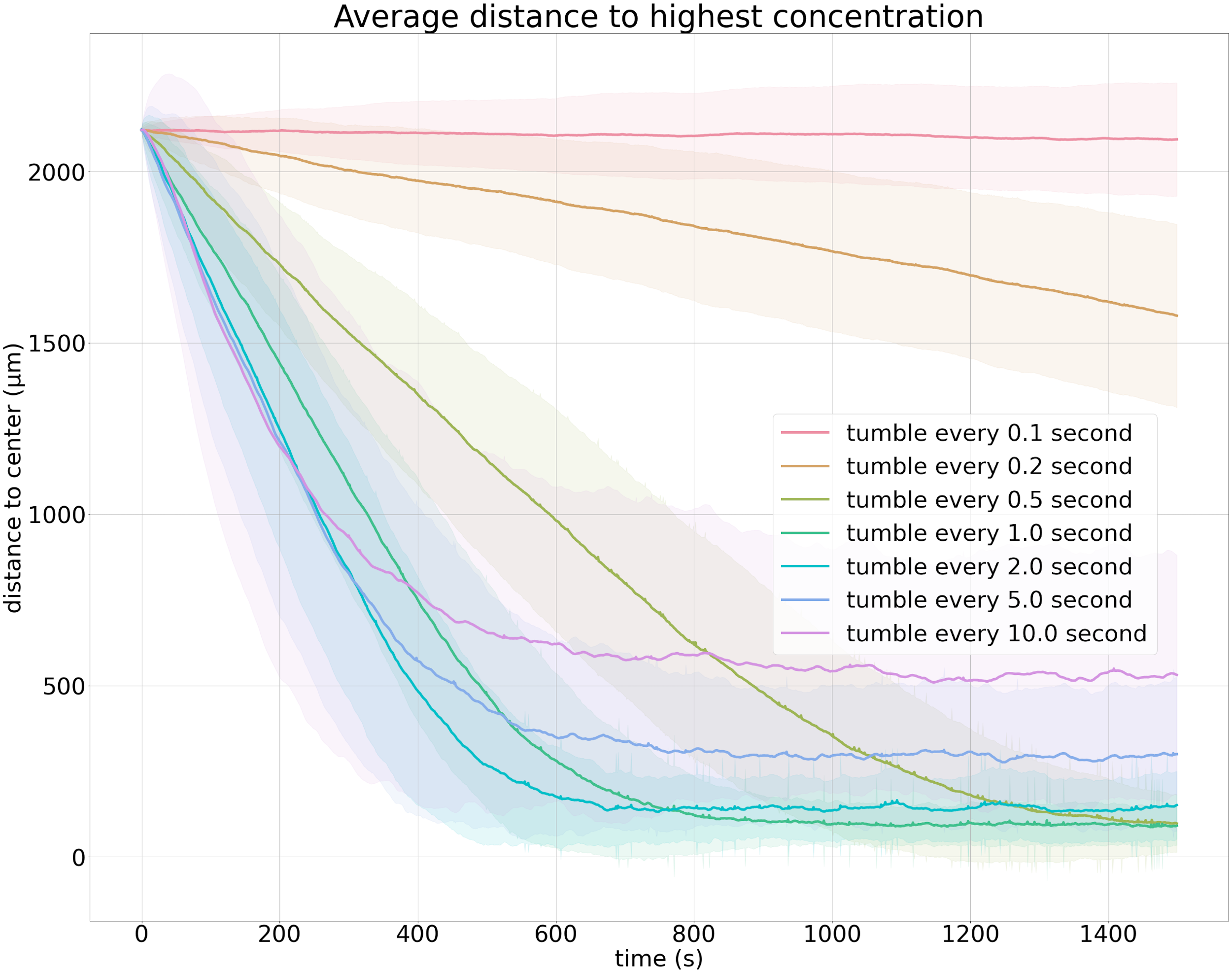 Average distance to the goal over time for 500 cells. Each colored line indicates the average distance to the goal over time for a different value of t0; the shaded area represents one standard deviation.
Below, we reproduce the video from earlier in this module showing E. coli moving towards a sugar crystal. This video shows that the behavior of real E. coli is similar to that of our simulated bacteria. Bacteria generally move towards the crystal and then remain close to it; some bacteria run by the crystal, but they turn around to move toward the crystal again.
Bacteria are even smarter than we thought
If you closely examine the video above, then you may be curious about the way that bacteria turn around and head back toward the attractant. When they reorient, their behavior appears more intelligent than simply walking in a random direction. As is often true in biology, the reality of the system that we are studying turns out to be more complex than we might at first imagine.
The direction of bacterial reorientation is not completely random, but rather follows a normal distribution with mean of 68° and standard deviation of 36°2. That is, the bacterium typically does not tend to make as drastic of a change to its orientation as it would in a pure random walk, which would have an average change in orientation of 90°.
Furthermore, the direction of the bacterium’s reorientation also depends on whether the cell is traveling in the correct direction.3 If the bacterium is moving up an attractant gradient, then it makes smaller changes in its reorientation angle, a feature that helps the cell continue moving straight if it is traveling in the direction of an attractant.
For that matter, the run-and-tumble model of E. coli only represents one way for bacteria to explore their surroundings. Microorganisms have many different sizes, shapes, metabolisms, and they live in a very diverse range of environments, which has produced several other exploration strategies.4.
We are fortunate to have this wealth of research on chemotaxis in E. coli, which may be the single most studied biological system from the perspective of understanding how chemical reactions produce emergent behavior. However, for the study of most biological systems, a clear thread connecting a reductionist view of the system to that system’s holistic behavior remains a dream. (For example: how can your thoughts while reading this parenthetical aside be distilled into the firings of individual neurons?) Fortunately, we can be confident that uncovering the underlying mechanisms of biological systems will continue to inspire the work of biological modelers for many years.
-
Saragosti J., Siberzan P., Buguin A. 2012. Modeling E. coli tumbles by rotational diffusion. Implications for chemotaxis. PLoS One 7(4):e35412. available online. ↩
-
Berg HC, Brown DA. 1972. Chemotaxis in Escherichia coli analysed by three-dimensional tracking. Nature. Available online ↩
-
Saragosti J, Calvez V, Bournaveas, N, Perthame B, Buguin A, Silberzan P. 2011. Directional persistence of chemotactic bacteria in a traveling concentration wave. PNAS. Available online ↩
-
Michell J.G., Kogure K. 2005. Bacterial motility: links to the environment and a driving force for microbial physics. FEMS Microbial Ecol 55:3-16. Available online ↩
