Software Tutorial: Adding Phosphorylation to our BioNetGen Model

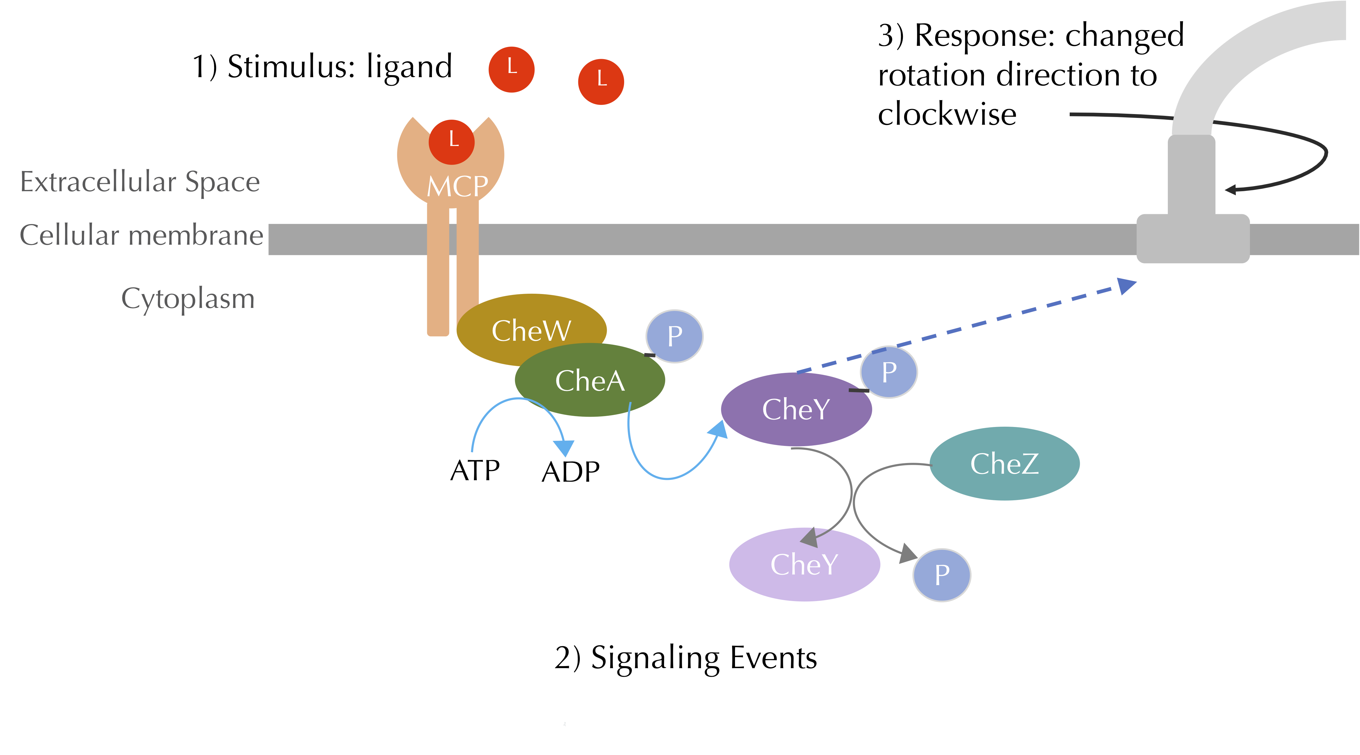
In this tutorial, we will extend the BioNetGen model covered in the ligand-receptor tutorial to add the phosphorylation chemotaxis mechanisms described in the main text, shown in the figure reproduced below.

To get started, open Visual Studio Code, and click File > Open Folder.... Open the EColiSimulations folder from the previous tutorial. Create a copy of your file from the ligand-receptor tutorial and save it as phosphorylation.bngl. If you would rather not follow along below, you can download a completed BioNetGen file here: phosphorylation.bngl

Defining molecules

Say that we wanted to specify all particles and the reactions involving them in the manner used up to this point in the book. We would need one particle type to represent MCP molecules, another particle type to represent ligands, and a third to represent bound complexes. A bound complex molecule binds with CheA and CheW and can be either phosphorylated or unphosphorylated, necessitating two different molecule types. In turn, CheY can be phosphorylated or unphosphorylated as well, requiring two more particles.

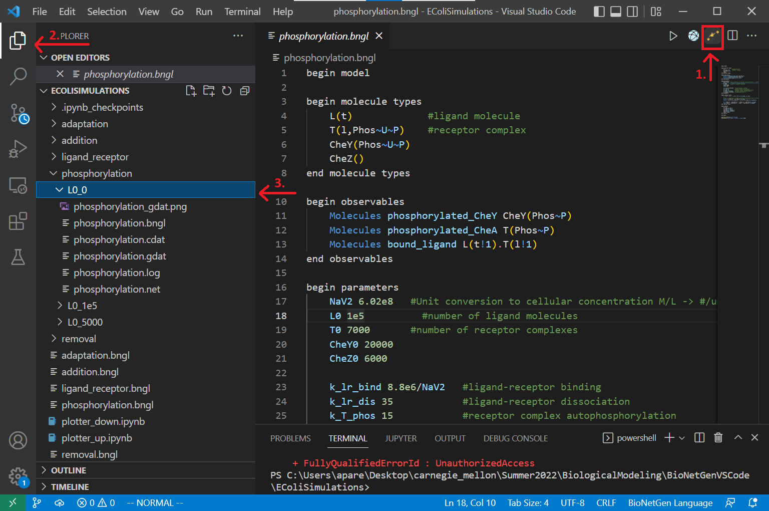
Instead, the BioNetGen language will allow us to conceptualize this system much more concisely using rules that apply to particles that are in a variety of states (we will say more about the paradigm of using rules soon in the main text). The BioNetGen representation of the four particles in our model is shown below. The notation Phos~U~P indicates that a given molecule type can be either phosphorylated or unphosphorylated, so that we do not need multiple different expressions to represent the molecule. We also add molecules CheY(Phos~U~P) and CheZ().

L(t)             #ligand molecule
T(l,Phos~U~P)    #receptor complex
CheY(Phos~U~P)
CheZ()

Note: Be careful with the use of spaces; don’t put spaces after the comma in the specification of the receptor.)

During this simulation, we are interested in tracking the concentration of phosphorylated CheY and CheA (receptor complex) along with the concentration of the ligand.

begin observables
	Molecules phosphorylated_CheY CheY(Phos~P)
	Molecules phosphorylated_CheA T(Phos~P)
	Molecules bound_ligand L(t!1).T(l!1)
end observables

Defining reactions

The conciseness of BioNetGen’s molecule representation helps us represent our reactions concisely as well. We first reproduce the reversible binding and dissociation reaction from the previous lesson.

LR: L(t) + T(l) <-> L(t!1).T(l!1) k_lr_bind, k_lr_dis

Next, we represent the phosphorylation of the MCP complex. Recall that the phosphorylation of CheA can occur at different rates depending on whether the MCP is bound, and so we will need two different reactions to model these different rates. In our model, the phosphorylation of the MCP will occur at one fifth the rate when it is bound to the attractant ligand.

FreeTP: T(l,Phos~U) -> T(l,Phos~P) k_T_phos
BoundTP: L(t!1).T(l!1,Phos~U) -> L(t!1).T(l!1,Phos~P) k_T_phos*0.2

Finally, we represent the phosphorylation and dephosphorylation of CheY. The former requires a phosphorylated MCP receptor, while the latter is done with the help of a CheZ molecule that can be in any state.

YP: T(Phos~P) + CheY(Phos~U) -> T(Phos~U) + CheY(Phos~P) k_Y_phos
YDep: CheZ() + CheY(Phos~P) -> CheZ() + CheY(Phos~U) k_Y_dephos

We use the snippets above to create a complete set of reaction rules for our simulated system.

begin reaction rules
	LigandReceptor: L(t) + T(l) <-> L(t!1).T(l!1) k_lr_bind, k_lr_dis

	#Free vs. ligand-bound complexes autophosphorylates
	FreeTP: T(l,Phos~U) -> T(l,Phos~P) k_T_phos
	BoundTP: L(t!1).T(l!1,Phos~U) -> L(t!1).T(l!1,Phos~P) k_T_phos*0.2

	YP: T(Phos~P) + CheY(Phos~U) -> T(Phos~U) + CheY(Phos~P) k_Y_phos
	YDep: CheZ() + CheY(Phos~P) -> CheZ() + CheY(Phos~U) k_Y_dephos
end reaction rules

Initializing molecules and parameters

To initialize our simulation, we need to indicate the number of molecules in each state present at the beginning of the simulation. Since we are adding ligands at the beginning of the simulation, the initial amount of molecules at each same state should be equal to the equilibrium concentrations when no ligand is present. To this end, we set the amount of phosphorylated receptor equal to one-fourth the concentration of unphosphorylated receptor, and the concentration of phosphorylated CheY to be equal to the concentration of unphosphorylated CheY.

Note: This was validated through trial and error.

begin species
	L(t) L0
	T(l,Phos~U) T0*0.8
	T(l,Phos~P) T0*0.2
	CheY(Phos~U) CheY0*0.5
	CheY(Phos~P) CheY0*0.5
	CheZ() CheZ0
end species

We now set initial quantities of molecules along with reaction rate parameters to be consistent with in vivo quantities ¹²³.

begin parameters
	NaV 6.02e8   #Unit conversion to cellular concentration M/L -> #/um^3
	L0 0        #number of ligand molecules
	T0 7000       #number of receptor complexes
	CheY0 20000
	CheZ0 6000

	k_lr_bind 8.8e6/NaV   #ligand-receptor binding
	k_lr_dis 35           #ligand-receptor dissociation
	k_T_phos 15           #receptor complex autophosphorylation
	k_Y_phos 3.8e6/NaV    #receptor complex phosphorylates CheY
	k_Y_dephos 8.6e5/NaV  #Z dephosphorylates CheY
end parameters

Note: The parameters section has to appear before the reaction rules section.

Place everything occurring above between begin model and end model tags.

Simulating responses to attractants

Before running the simulation, let’s think about what will happen. If we don’t add any ligand molecule into the system, then assuming that we have started the simulation at steady state, then the concentrations of phosphorylated receptors and CheY will remain at equilibrium.

We can now run the simulation, setting t_end equal to 3 in order to run the simulation for longer than we did in the ligand-receptor tutorial. Place the following code after end model in your BioNetGen file.

generate_network({overwrite=>1})
simulate({method=>"ssa", t_end=>3, n_steps=>100})

The following code contains our complete simulation, which you can also download here: phosphorylation.bngl

begin model

begin molecule types
	L(t)             #ligand molecule
	T(l,Phos~U~P)    #receptor complex
	CheY(Phos~U~P)
	CheZ()
end molecule types

begin observables
	Molecules phosphorylated_CheY CheY(Phos~P)
	Molecules phosphorylated_CheA T(Phos~P)
	Molecules bound_ligand L(t!1).T(l!1)
end observables

begin parameters
	NaV2 6.02e8   #Unit conversion to cellular concentration M/L -> #/um^3
	L0 5e3          #number of ligand molecules
	T0 7000       #number of receptor complexes
	CheY0 20000
	CheZ0 6000

	k_lr_bind 8.8e6/NaV2   #ligand-receptor binding
	k_lr_dis 35            #ligand-receptor dissociation
	k_T_phos 15            #receptor complex autophosphorylation
	k_Y_phos 3.8e6/NaV2    #receptor complex phosphorylates Y
	k_Y_dephos 8.6e5/NaV2  #Z dephosphorylates Y
end parameters

begin reaction rules
	LR: L(t) + T(l) <-> L(t!1).T(l!1) k_lr_bind, k_lr_dis

	#Free vs. ligand-bound receptor complexes autophosphorylates at different rates
	FreeTP: T(l,Phos~U) -> T(l,Phos~P) k_T_phos
	BoundTP: L(t!1).T(l!1,Phos~U) -> L(t!1).T(l!1,Phos~P) k_T_phos*0.2

	YP: T(Phos~P) + CheY(Phos~U) -> T(Phos~U) + CheY(Phos~P) k_Y_phos
	YDep: CheZ() + CheY(Phos~P) -> CheZ() + CheY(Phos~U) k_Y_dephos
end reaction rules

begin species
	L(t) L0
	T(l,Phos~U) T0*0.8
	T(l,Phos~P) T0*0.2
	CheY(Phos~U) CheY0*0.5
	CheY(Phos~P) CheY0*0.5
	CheZ() CheZ0
end species

end model

generate_network({overwrite=>1})
simulate({method=>"ssa", t_end=>3, n_steps=>100})

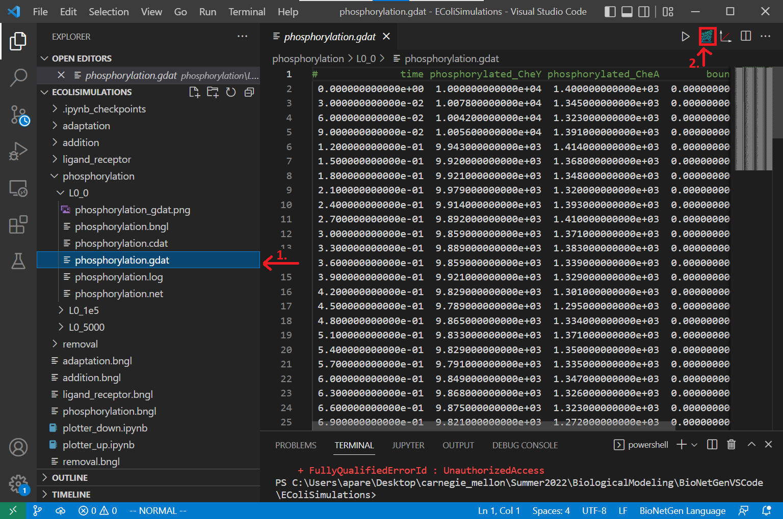
Now save your file and run the simulation by clicking the Run BNG button. The results will be saved in a new folder called phosphorylation/TIMESTAMP contained in the current directory. Rename the folder within phosphorylation from the time stamp to L0.

Open the newly created phosphorylation.gdat file within this folder, and plot the data by clicking on Built-in plotting. What do you observe?

When we add ligand molecules into the system, as we did in the tutorial for ligand-receptor dynamics, the concentration of bound receptors should increase. What will happen to the concentration of phosphorylated CheA, and phosphorylated CheY? What will happen to steady state concentrations?

Now run your simulation by changing L0 to be equal to 5000 and then run it again with L0 to be equal to 1e5. Do the results confirm your hypothesis? What happens as we keep changing L0? What happens as L0 gets really large (e.g., 1e9)? What do you think is going on?

In the main text, we will explore the results of the above simulation. We will then interpret how differences in the amounts of initial ligand can influence changes in the concentration of phosphorylated CheY (and therefore the bacterium’s tumbling frequency).

Return to main text

Li M, Hazelbauer GL. 2004. Cellular stoichimetry of the components of the chemotaxis signaling complex. Journal of Bacteriology. Available online ↩
Spiro PA, Parkinson JS, and Othmer H. 1997. A model of excitation and adaptation in bacterial chemotaxis. Biochemistry 94:7263-7268. Available online. ↩
Stock J, Lukat GS. 1991. Intracellular signal transduction networks. Annual Review of Biophysics and Biophysical Chemistry. Available online ↩

Defining molecules

Defining reactions

Initializing molecules and parameters

Simulating responses to attractants

Comments