Methylation Helps a Bacterium Adapt to Differing Concentrations

Bacterial tumbling frequencies remain constant for different attractant concentrations

In the previous lesson, we explored the signal transduction pathway by which E. coli can change its tumbling frequency in response to a change in the concentration of an attractant. But the reality of cellular environments is that the concentration of an attractant can vary across several orders of magnitude. The cell therefore needs to detect not absolute concentrations of an attractant but rather relative changes.

E. coli detects relative changes in its concentration via adaptation to these changes. If the concentration of attractant remains constant for a period of time, then regardless of the absolute value of the concentration, the cell returns to the same background tumbling frequency. That is, E. coli demonstrates robustness to the attractant concentration in maintaining its default tumbling behavior.

However, our current model is not able to address this adaptation. If the ligand concentration increases in the model, then phosphorylated CheY will plummet and remain at a low steady state.

In this lesson, we will investigate the biochemical mechanism that E. coli uses to achieve such a robust response to environments with different background concentrations. We will then expand the model we built in the previous lesson to replicate the bacterium’s adaptive response.

Bacteria remember past concentrations using methylation

Recall that in the absence of an attractant, CheW and CheA readily bind to an MCP, leading to greater autophosphorylation of CheA, which in turn phosphorylates CheY. The greater the concentration of phosphorylated CheY, the more frequently the bacterium tumbles.

Signal transduction is achieved through phosphorylation, but E. coli maintains a “memory” of past environmental concentrations through a chemical process called methylation. In this reaction, a methyl group (-CH₃) is added to an organic molecule; the removal of a methyl group is called demethylation.

Every MCP receptor contains four methylation sites, meaning that between zero and four methyl groups can be added to the receptor. On the plasma membrane, many MCPs, CheW, and CheA molecules form an array structure. Methylation reduces the negative charge on the receptors, stabilizing the array and facilitating CheA autophosphorylation. The more sites that are methylated, the higher the autophosphorylation rate of CheA, which means that CheY has a higher phosphorylation rate, and tumbling frequency increases.

We now have two different ways that tumbling frequency can be elevated. First, if the concentration of an attractant is low, then CheW and CheA freely form a complex with the MCP, and the phosphorylation cascade passes phosphoryl groups to CheY, which interacts with the flagella and keeps tumbling frequency high. Second, an increase in MCP methylation can also boost CheA autophosphorylation and lead to increased tumbling frequency.

Methylation of MCPs is achieved by an additional protein called CheR. When bound to MCPs, CheR methylates ligand-bound MCPs faster¹², and so the rate of MCP methylation by CheR is higher if the MCP is bound to a ligand.³. Let’s consider how this fact affects a bacterium’s behavior.

Say that E. coli encounters an increase in attractant concentration. Then the lack of a phosphorylation cascade will mean less phosphorylated CheY, and so the tumbling frequency will decrease. However, if the attractant concentration levels off, then the tumbling frequency will flatten, while CheR starts methylating the MCP. Over time, the rising methylation will increase CheA autophosphorylation, bringing back the phosphorylation cascade and raising tumbling frequency back to default levels.

Just as the phosphorylation of CheY can be reversed, MCP methylation can be undone to prevent methylation from being permanent. In particular, an enzyme called CheB, which like CheY is phosphorylated by CheA, demethylates MCPs (as well as autodephosphorylates). The rate of an MCP’s demethylation is dependent on the extent to which the MCP is methylated. In other words, the rate of MCP methylation is higher when the MCP is in a low methylation state, and the rate of demethylation is faster when the MCP is in a high methylation state.³

The figure below adds CheR and CheB to provide a complete picture of the core pathways influencing chemotaxis. To model these pathways and see how our simulated bacterial system responds to different relative attractant concentrations, we will need to add quite a few molecules and reactions to our current model.

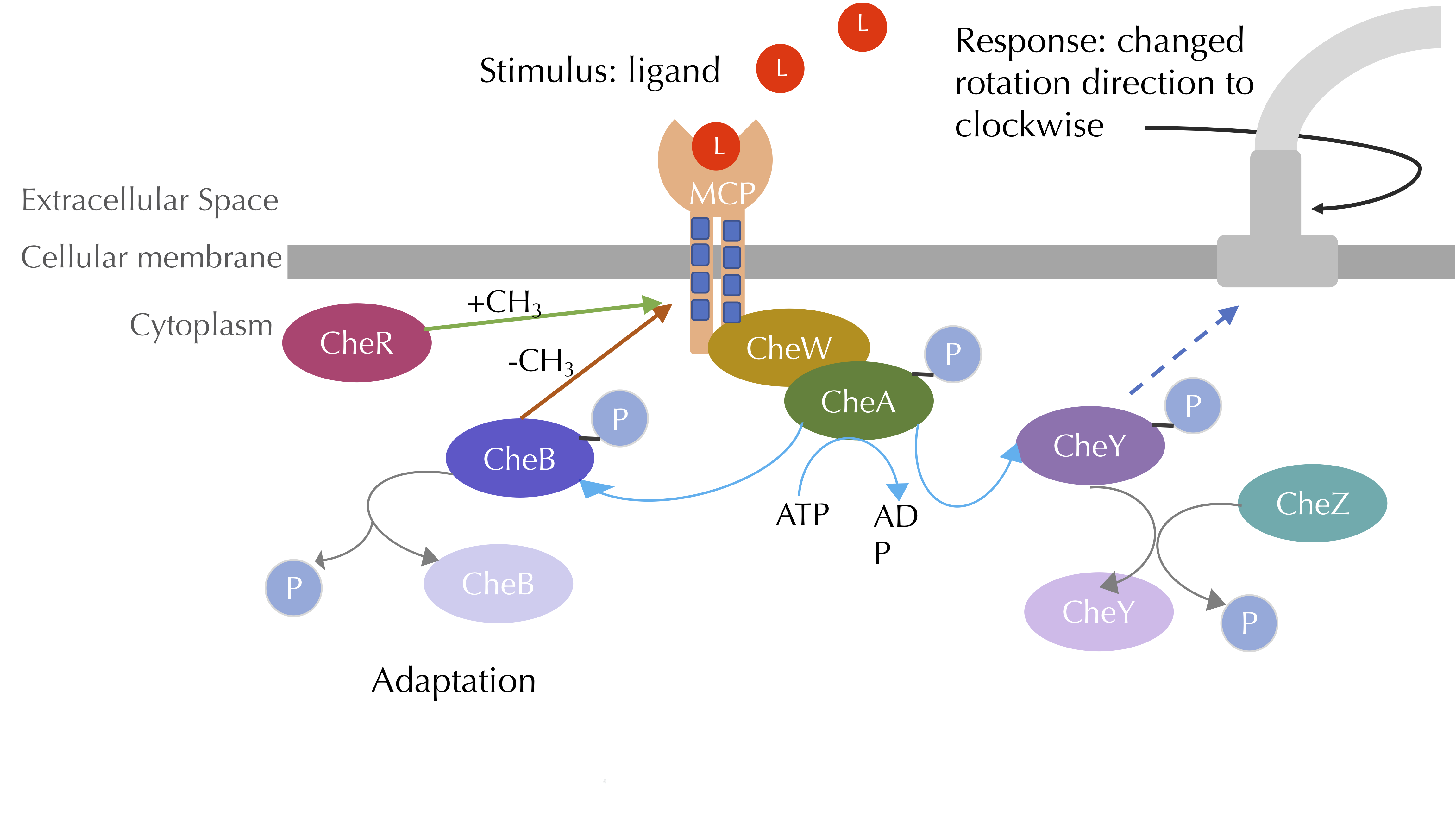The chemotaxis signal-transduction pathway with methylation included. CheA phosphorylates CheB, which methylates MCPs, while CheR demethylates MCPs. Blue lines denote phosphorylation, grey lines denote dephosphorylation, green arrows denote methylation, and red arrows denote demethlyation. Image modified from Parkinson Lab’s illustrations.

Combinatorial explosion and the need for rule-based modeling

To expand our model, we will need to include methylation of the MCP by CheR and demethylation of the MCP by CheB. For simplicity, we will use three methylation levels (low, medium, and high) rather than five.

Imagine that we were attempting to specify every reaction that could take place in our model. To specify an MCP, we would need to establsh whether it is bound to a ligand (two possible states), whether it is bound to CheR (two possible states), whether it is phosphorylated (two possible states), and which methylation state it is in (three possible states). Therefore, a given MCP would need 2 · 2 · 2 · 3 = 24 total states.

Consider the simple reaction of a ligand binding to an MCP, which we originaly wrote as T + L → TL. We now need this reaction to include 12 of the 24 states, the ones corresponding to the MCP being unbound to the ligand. Our previously simply reaction would become, 12 different reactions, one for each possible unbound state of the complex molecule T. And if the situation were just a little more complex, with the ligand molecule L having n possible states, then we would have 12n reactions. Image trying to debug a model in which we had accidentally incorporated a type when transcribing just one of these reaction!

In other words, as our model grows, with multiple different states for each molecule involved in each reaction, the number of reactions that we need to represent the system grows rapidly; this phenomenon is called combinatorial explosion and means that building realistic models of biochemical systems at scale can be daunting.

Yet all these 12 reactions can be summarized with a single rule: a ligand and a receptor can bind into a complex if the receptor is unbound. Moreover, all 12 reactions implied by the rule are easily inferable from it. This example illustrates rule-based modeling, a paradigm applied by BioNetGen in which a potentially enormous number of reactions are specified by a much smaller collection of “rules” from which all reactions can be inferred.

We will not bog down the main text with a full specification of all the rules needed to add methylation to our model while avoiding combinatorial explosion. If you are interested in the details, please follow our tutorial.

Visit tutorial

Bacterial tumbling is robust to large sudden changes in attractant concentration

In the figures that follow, we plot the concentration over time of each molecule for different values of l₀, the initial concentration of ligand. From what we have learned about E. coli, we should see the concentration of phosphorylated CheY (and therefore the bacterium’s tumbling frequency) drop before returning to its original equilibrium. But will our simulation capture this behavior?

First, we add a relatively small amount of attractant, setting l₀ equal to 10,000. The system returns so quickly to an equilibrium in phosphorylated CheY that it is difficult to imagine that the attractant has had any effect on tumbling frequency.

Molecular concentrations (in number of molecules in the cell) over time (in seconds) in a BioNetGen chemotaxis simulation with 10,000 initial attractant ligand particles.

If instead l₀ is equal to 100,000, then we obtain the figure below. After an initial drop in the concentration of phosphorylated CheY, it returns to equilibrium after a few minutes.

Molecular concentrations (in number of molecules in the cell) over time (in seconds) in a BioNetGen chemotaxis simulation with 100,000 initial attractant ligand particles.

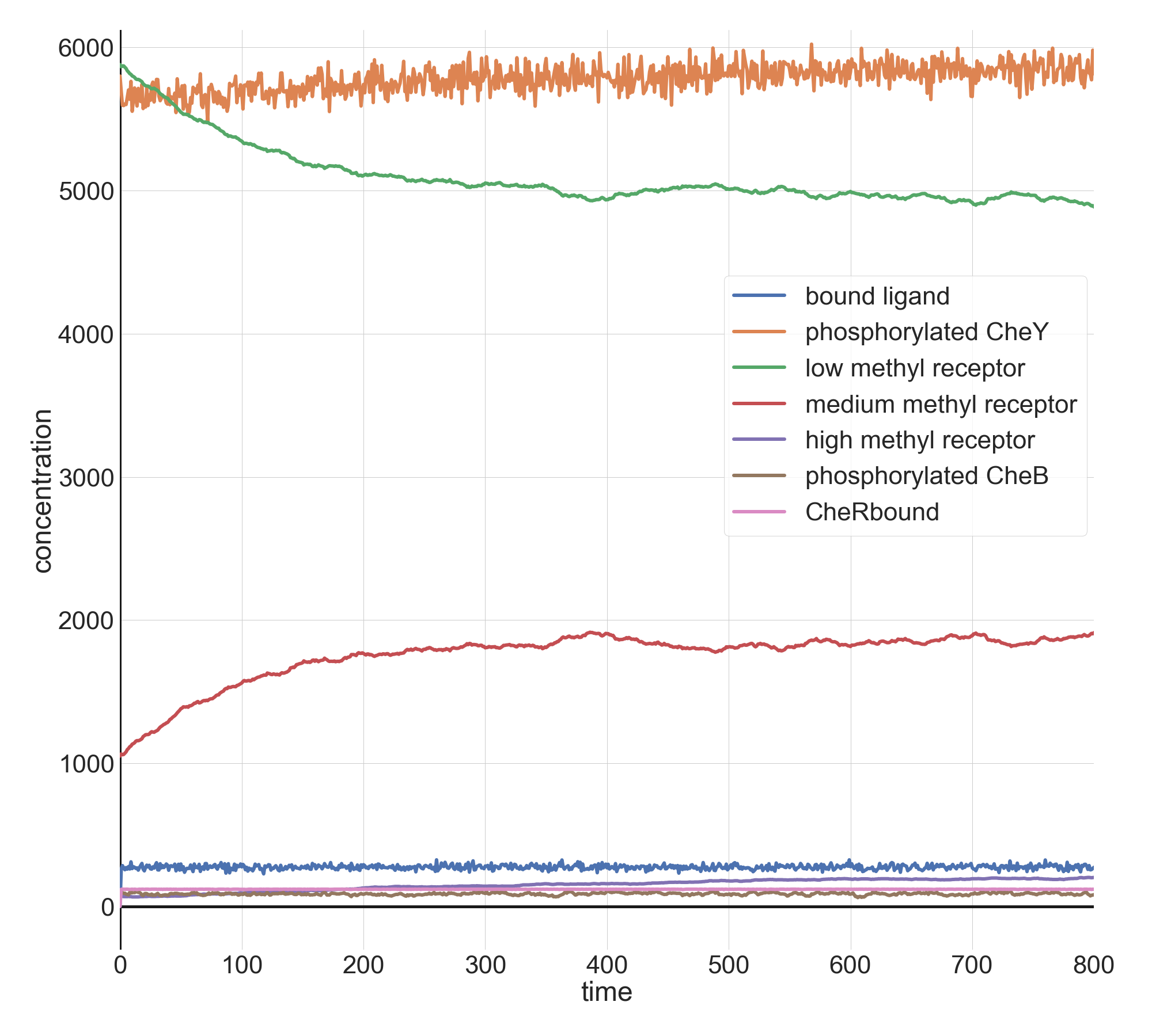
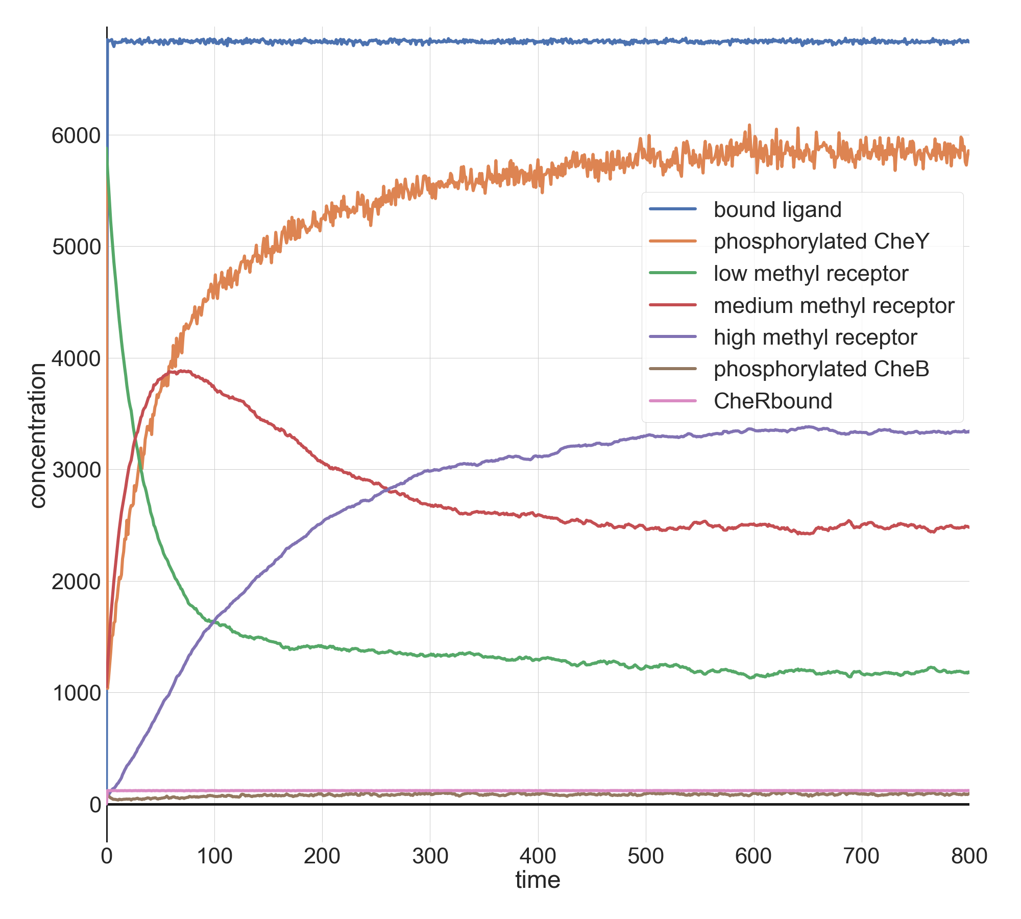
When we increase l₀ by another factor of ten to 1 million, the initial drop is more pronounced, but the system returns just as quickly to equilibrium. Note how much higher the concentration of methylated receptors are in this figure compared to the previous figure; however, there are still a significant concentration of receptors with low methylation, indicating that the system may be able to handle an even larger jolt of attractant.

Molecular concentrations (in number of molecules in the cell) over time (in seconds) in a BioNetGen chemotaxis simulation with one million initial attractant ligand particles.

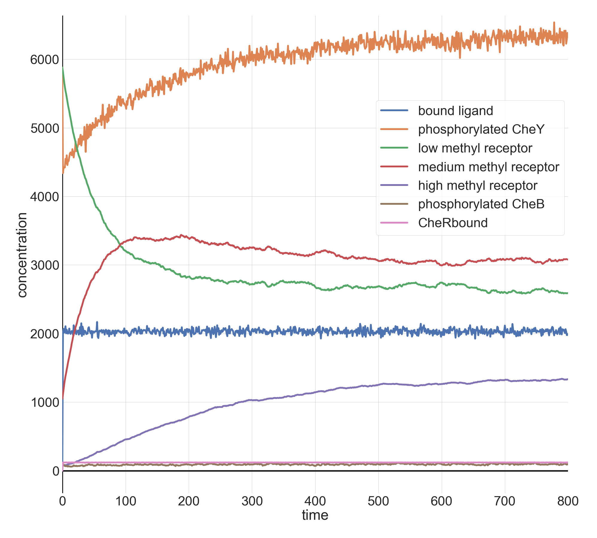
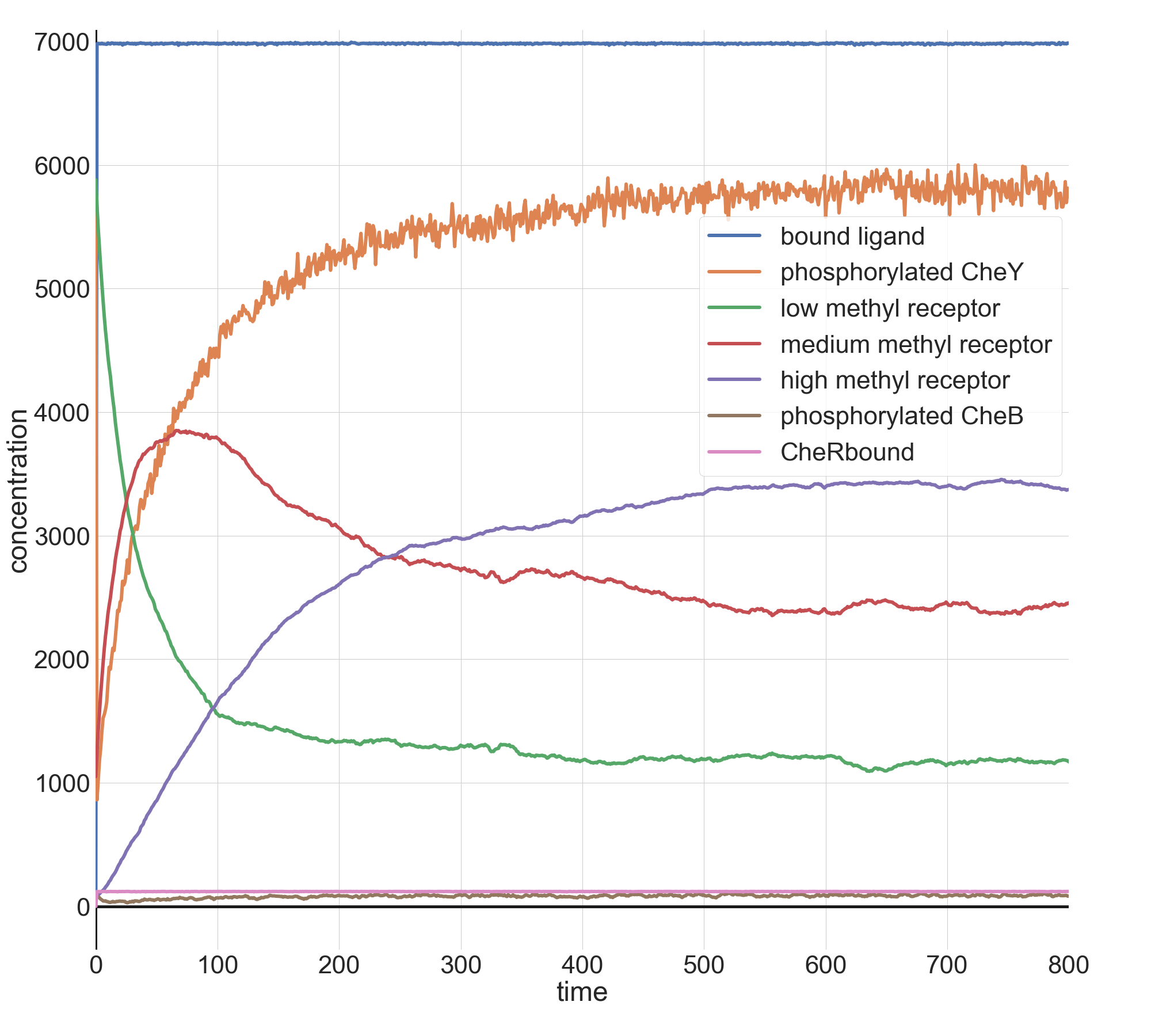
When we set l₀ equal to 10 million, we give the system this bigger jolt. Once again, the model returns to its previous CheY equilibrium after a few minutes.

Molecular concentrations (in number of molecules in the cell) over time (in seconds) in a BioNetGen chemotaxis simulation with ten million initial attractant ligand particles.

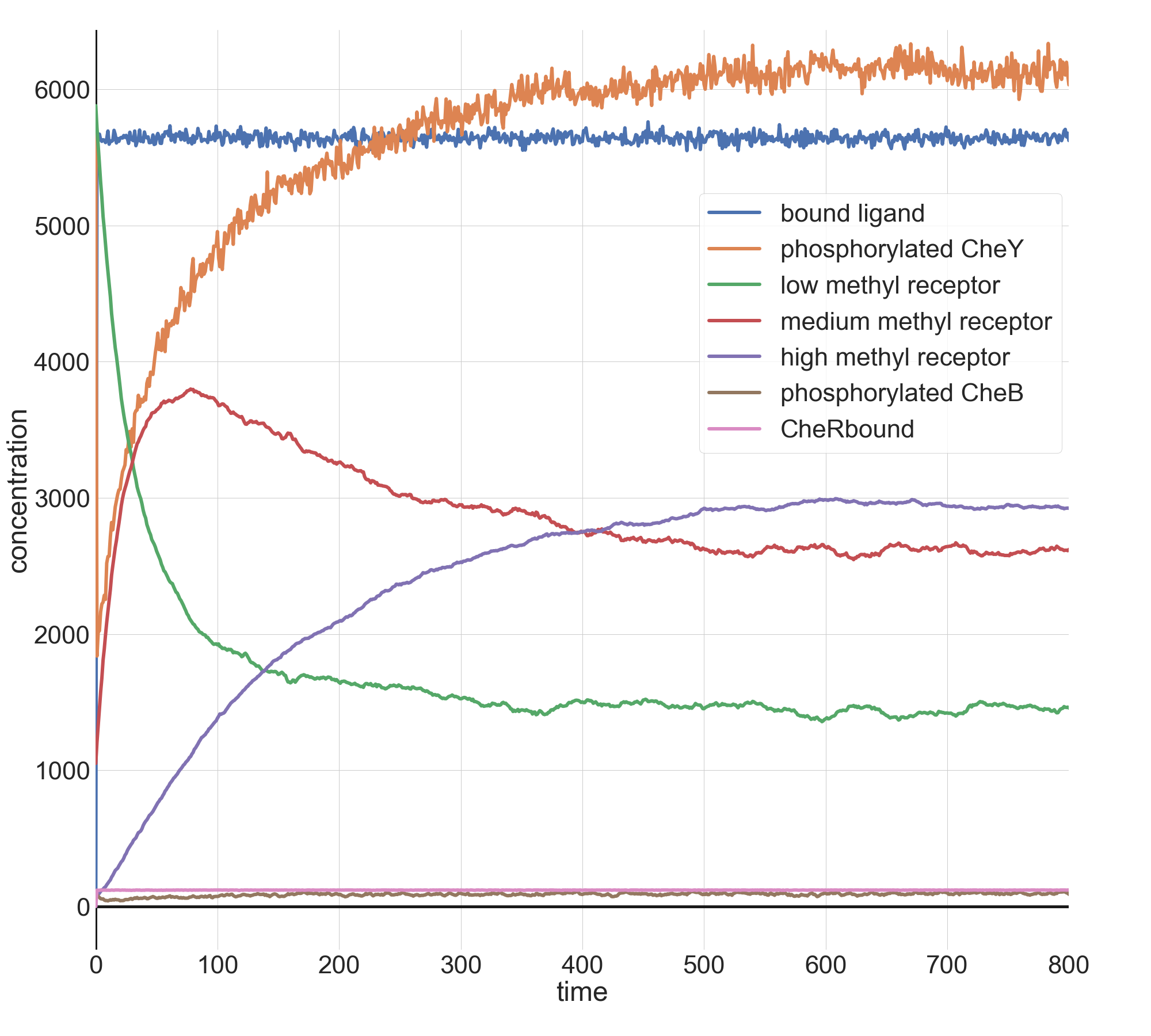
Finally, with l₀ equal to 100 million, we see what we might expect: the steepest drop in phosphorylated CheY yet, but a system that is able to return to equilibrium after a few minutes.

Molecular concentrations (in number of molecules in the cell) over time (in seconds) in a BioNetGen chemotaxis simulation with 100 million initial attractant ligand particles.

Our model, which is built on real reaction rate parameters, provides compelling evidence that the E. coli chemotaxis system is robust to changes in its environment across several orders of magnitude of attractant concentration. This robustness has been observed in real bacteria⁴⁵, as well as replicated by other computational simulations⁶.

Aren’t bacteria magnificent?

Traveling up an attractant gradient

We have simulated E. coli adapting to a single sudden change in its environment, but life often depends on responding to continual change. Imagine a glucose cube in an aqueous solution. As the cube dissolves, a gradient will form, with a glucose concentration that decreases outward from the cube. How will the tumbling frequency of E. coli change if the bacterium finds itself in an environment of an attractant gradient? Will the tumbling frequency decrease continuously as well, or will we see more complicated behavior? And once the cell reaches a region of high attractant concentration, will its default tumbling frequency stabilize to the same steady state?

We will modify our model by increasing the concentration of the attractant ligand exponentially and seeing how the concentration of phosphorylated CheY changes. This model will simulate a bacterium traveling up an attractant gradient toward an attractant. Moreover, we will examine how the concentration of phosphorylated CheY changes as we change the gradient’s “steepness”, or the rate at which attractant ligand is increasing. Visit the following tutorial if you’re interested in following our adjustments for yourself.

Visit tutorial

Steady state tumbling frequency is robust

To model a ligand concentration [L] that is increasing exponentially, we will use the function [L] = l₀ · e^{k · t}, where e is Euler’s number (e = 2.71828…) l₀ is the initial ligand concentration, k is a constant dictating the rate of exponential growth, and t is time. The parameter k represents the steepness of the gradient, since the higher the value of k, the faster the growth in the ligand concentration [L].

For example, the following figure shows the concentration over time of phosphorylated CheY (orange) when l₀ = 1000 and k = 0.1. The concentration of phosphorylated CheY, and therefore the tumbling frequency, still decreases sharply as the ligand concentration increases, but after all ligands become bound to receptors (the plateau in the blue curve), receptor methylation causes the concentration of phosphorylated CheY to return to its equilibrium. For these values of l₀ and k, the outcome is similar to when we provided an instantaneous increase in ligand, although the cell takes longer to reach its minimum concentration of phosphorylated CheY because the attractant concentration is increasing gradually.

Plots of relevant molecule concentrations in our model (in number of molecules in the cell) over time (in seconds) when the concentration of ligand grows exponentially with l₀ = 1000 and k = 0.1. The concentration of bound ligand (shown in red) quickly hits saturation, which causes a minimum in phosphorylated CheY (orange), and therefore a low tumbling frequency. To respond, the cell increases the methylation of receptors, which boosts the concentration of phosphorylated CheY back to equilibrium.

The following figure shows the results of multiple simulations in which we vary the growth parameter k and plot only the concentration of phosphorylated CheY over time. The larger the value of k, the faster the increase in receptor binding, and the steeper the drop in the concentration of phosphorylated CheY.

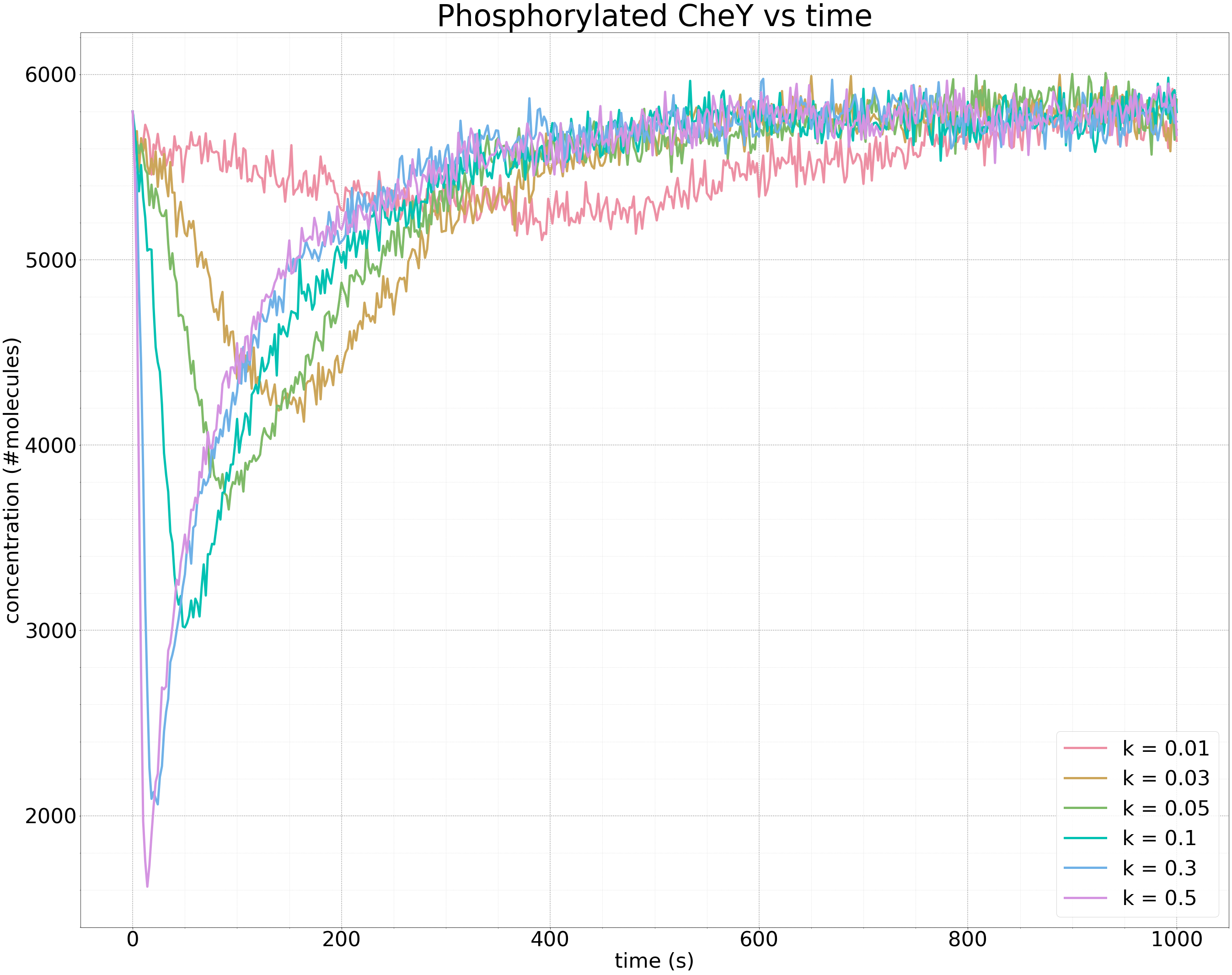Plots of the concentration of phosphorylated CheY over time (in seconds) for different growth rates k of ligand concentration. The larger the value of k, the steeper the initial drop in the concentration of phosphorylated CheY, and the faster that methylation returns the concentration of phosphorylated CheY to equilibrium. The same equilibrium is obtained regardless of the value of k.

The above figure further illustrates the robustness of bacterial chemotaxis to the rate of growth in ligand concentration. Whether the growth of the attractant is slow or fast, methylation will always bring the cell back to the same equilibrium concentration of phosphorylated CheY and therefore the same background tumbling frequency.

From changing tumbling frequencies to an exploration algorithm

We hope that our work here has conveyed the elegance of bacterial chemotaxis, as well as the power of rule-based modeling and the Gillespie algorithm for simulating a complex biochemical system that may include a huge number of reactions.

And yet we are missing an important part of the story. E. coli has evolved to ensure that if it detects a relative increase in concentration (i.e., an attractant gradient), then it can reduce its tumbling frequency in response. But we have not explored why changing its tumbling frequency would help a bacterium find food in the first place. After all, according to the run and tumble model, the direction that a bacterium is moving at any point in time is random!

This quandary does not have an obvious intuitive answer. In this module’s conclusion, we will build a model to explain why E. coli’s randomized run and tumble walk algorithm is a clever way of locating resources in an unfamiliar land.

Next lesson

Additional resources

If you find chemotaxis biology as interesting as we do, then we suggest the following resources.

• An amazing introduction to chemotaxis from the Parkinson Lab.
• A good overview of chemotaxis: Webre et al. 2003
• A review article on chemotaxis pathway and MCPs: Baker et al. 2005.
• A more recent review article of MCPs: Parkinson et al. 2015.
• Lecture notes on robustness and integral feedback: Berg 2008.

1. Amin DN, Hazelbauer GL. 2010. Chemoreceptors in signaling complexes: shifted conformation and asymmetric coupling. Available online ↩

2. Terwilliger TC, Wang JY, Koshland DE. 1986. Kinetics of Receptor Modification - the multiply methlated aspartate receptors involved in bacterial chemotaxis. The Journal of Biolobical Chemistry. Available online ↩

3. Spiro PA, Parkinson JS, and Othmer H. 1997. A model of excitation and adaptation in bacterial chemotaxis. Biochemistry 94:7263-7268. Available online. ↩ ↩²

4. Shimizu TS, Delalez N, Pichler K, and Berg HC. 2005. Monitoring bacterial chemotaxis by using bioluminescence resonance energy transfer: absence of feedback from the flagellar motors. PNAS. Available online ↩

5. Krembel A., Colin R., Sourijik V. 2015. Importance of multiple methylation sites in Escherichia coli chemotaxis. Available online ↩

6. Bray D, Bourret RB, Simon MI. 1993. Computer simulation of phosphorylation cascade controlling bacterial chemotaxis. Molecular Biology of the Cell. Available online ↩