Software Tutorial: Traveling Up an Attractant Gradient

In the previous tutorial, we modeled how bacteria react and adapt to a one-time addition of attractants. In real life, bacteria don’t suddenly drop into an environment with more attractants; instead, they explore a variable environment. In this tutorial, we will adapt our model to simulate a bacterium as it travels up an exponentially increasing concentration gradient.

We will also explore defining and using functions, a feature of BioNetGen that will allow us to specify reaction rules in which the reaction rates are dependent on the current state of the system.

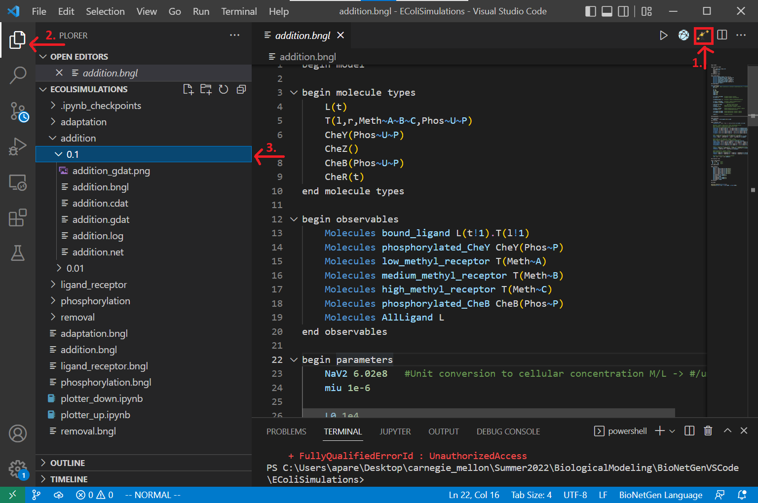
To get started, open Visual Studio Code, and click File > Open Folder.... Open the EColiSimulations folder from the first tutorial. Create a copy of your adaptation.bngl file from the adaptation tutorial and save it as addition.bngl. If you would rather not follow along below, you can download a completed BioNetGen file here: addition.bngl

We also will build a Jupyter notebook in this tutorial for plotting the concentrations of molecules over time. You should create a file called plotter_up.ipynb; if you would rather not follow along, we provide a completed notebook here: plotter_up.ipynb

Before running this notebook, make sure the following dependencies are installed.

Installation Link	Version	Check install/version
Python3	3.6+	python --version
Jupyter Notebook	4.4.0+	jupyter --version
Numpy	1.14.5+	pip list \| grep numpy
Matplotlib	3.0+	pip list \| grep matplotlib
Colorspace or with pip	any	pip list \| grep colorspace

Modeling an increasing ligand gradient with a BioNetGen function

Our BioNetGen model will largely stay the same, except for the fact that we are changing the concentration of ligand over time. To model an increasing concentration of ligand corresponding to a bacterium moving up an attractant gradient, we will increase the background ligand concentration at an exponential rate.

We will simulate an increase in attractant concentration by using a “dummy reaction” L → 2L in which one ligand molecule becomes two. To do so, we will add the following reaction to the reaction rules section.

As we have observed earlier in this module, when the ligand concentration is very high, receptors are saturated, and the cell can no longer detect a change in ligand concentration. If you explored the adaptation simulation, then you saw that this occurs after l₀ passes 1e8; we will therefore cap the allowable ligand concentration at this value.

We can cap our ligand concentration by defining the rate of the dummy reaction using a function add_Rate(). This function requires another observable, AllLigand. By adding the line Molecules AllLigand L in the observables section, AllLigand will record the total concentration of ligand in the system at each time step (both bound and unbound). As for our reaction, if AllLigand is less than 1e8, then the dummy reaction should take place at some given rate k_add. Otherwise, AllLigand exceeds1e8, and we will set the rate of the dummy reaction to zero. This can be achieved with a functions section in BioNetGen using the following if statement to branch based on the value of AllLigand.

Note: Please ensure that the functions section occurs before the reaction rules section in your BioNetGen file.

begin functions
	addRate() = if(AllLigand>1e8,0,k_add)
end functions

Now we are ready to add our dummy reaction to the reaction rules section with a reaction rate of addRate().

#Simulate an exponentially increasing gradient using a dummy reaction
LAdd: L(t) -> L(t) + L(t) addRate()

Now that we have defined our dummy reaction, we should specify the default rate of this reaction k_add in the parameters section. We first will try a value of k_add of 0.1/s with an initial ligand concentration L0 of 1e4. This means that the model is simulating a gradient of d[L]/dt = 0.1[L]. If L0 is 1e4, then the solution to this differential equation is [L] = 1000e^0.1t molecules per second.

k_add 0.1
L0 1e4

Running our updated BioNetGen model

Because we have largely kept the same model from the adaptation tutorial, we are ready to simulate. Please make sure that the following lines appear after end model so that we can run our simulation for 1000 seconds.

generate_network({overwrite=>1})
simulate({method=>"ssa", t_end=>1000, n_steps=>500})

The following code contains our complete simulation, which you can also download here: addition.bngl

begin model

begin molecule types
	L(t)
	T(l,r,Meth~A~B~C,Phos~U~P)
	CheY(Phos~U~P)
	CheZ()
	CheB(Phos~U~P)
	CheR(t)
end molecule types

begin observables
	Molecules bound_ligand L(t!1).T(l!1)
	Molecules phosphorylated_CheY CheY(Phos~P)
	Molecules low_methyl_receptor T(Meth~A)
	Molecules medium_methyl_receptor T(Meth~B)
	Molecules high_methyl_receptor T(Meth~C)
	Molecules phosphorylated_CheB CheB(Phos~P)
	Molecules AllLigand L
end observables

begin parameters
	NaV2 6.02e8   #Unit conversion to cellular concentration M/L -> #/um^3
	miu 1e-6

	L0 1e4
	T0 7000
	CheY0 20000
	CheZ0 6000
	CheR0 120
	CheB0 250

	k_lr_bind 8.8e6/NaV2   #ligand-receptor binding
	k_lr_dis 35            #ligand-receptor dissociation

	k_TaUnbound_phos 7.5   #receptor complex autophosphorylation

	k_Y_phos 3.8e6/NaV2    #receptor complex phosphorylates Y
	k_Y_dephos 8.6e5/NaV2  #Z dephosphorylates Y

	k_TR_bind 2e7/NaV2          #Receptor-CheR binding
	k_TR_dis  1            #Receptor-CheR dissociaton
	k_TaR_meth 0.08        #CheR methylates receptor complex

	k_B_phos 1e5/NaV2      #CheB phosphorylation by receptor complex
	k_B_dephos 0.17        #CheB autodephosphorylation

	k_Tb_demeth 5e4/NaV2   #CheB demethylates receptor complex
	k_Tc_demeth 2e4/NaV2   #CheB demethylates receptor complex

	k_add 0.1              #Ligand increase

end parameters

begin functions
	addRate() = if(AllLigand>1e8,0,k_add)
end functions

begin reaction rules
	LigandReceptor: L(t) + T(l) <-> L(t!1).T(l!1) k_lr_bind, k_lr_dis

	#Receptor complex (specifically CheA) autophosphorylation
	#Rate dependent on methylation and binding states
	#Also on free vs. bound with ligand
	TaUnboundP: T(l,Meth~A,Phos~U) -> T(l,Meth~A,Phos~P) k_TaUnbound_phos
	TbUnboundP: T(l,Meth~B,Phos~U) -> T(l,Meth~B,Phos~P) k_TaUnbound_phos*1.1
	TcUnboundP: T(l,Meth~C,Phos~U) -> T(l,Meth~C,Phos~P) k_TaUnbound_phos*2.8
	TaLigandP: L(t!1).T(l!1,Meth~A,Phos~U) -> L(t!1).T(l!1,Meth~A,Phos~P) 0
	TbLigandP: L(t!1).T(l!1,Meth~B,Phos~U) -> L(t!1).T(l!1,Meth~B,Phos~P) k_TaUnbound_phos*0.8
	TcLigandP: L(t!1).T(l!1,Meth~C,Phos~U) -> L(t!1).T(l!1,Meth~C,Phos~P) k_TaUnbound_phos*1.6

	#CheY phosphorylation by T and dephosphorylation by CheZ
	YPhos: T(Phos~P) + CheY(Phos~U) -> T(Phos~U) + CheY(Phos~P) k_Y_phos
	YDephos: CheZ() + CheY(Phos~P) -> CheZ() + CheY(Phos~U) k_Y_dephos

	#CheR binds to and methylates receptor complex
	#Rate dependent on methylation states and ligand binding
	TRBind: T(r) + CheR(t) <-> T(r!2).CheR(t!2) k_TR_bind, k_TR_dis
	TaRUnboundMeth: T(r!2,l,Meth~A).CheR(t!2) -> T(r,l,Meth~B) + CheR(t) k_TaR_meth
	TbRUnboundMeth: T(r!2,l,Meth~B).CheR(t!2) -> T(r,l,Meth~C) + CheR(t) k_TaR_meth*0.1
	TaRLigandMeth: T(r!2,l!1,Meth~A).L(t!1).CheR(t!2) -> T(r,l!1,Meth~B).L(t!1) + CheR(t) k_TaR_meth*30
	TbRLigandMeth: T(r!2,l!1,Meth~B).L(t!1).CheR(t!2) -> T(r,l!1,Meth~C).L(t!1) + CheR(t) k_TaR_meth*3

	#CheB is phosphorylated by receptor complex, and autodephosphorylates
	CheBphos: T(Phos~P) + CheB(Phos~U) -> T(Phos~U) + CheB(Phos~P) k_B_phos
	CheBdephos: CheB(Phos~P) -> CheB(Phos~U) k_B_dephos

	#CheB demethylates receptor complex
	#Rate dependent on methyaltion states
	TbDemeth: T(Meth~B) + CheB(Phos~P) -> T(Meth~A) + CheB(Phos~P) k_Tb_demeth
	TcDemeth: T(Meth~C) + CheB(Phos~P) -> T(Meth~B) + CheB(Phos~P) k_Tc_demeth

	#Simulate exponentially increasing gradient
	LAdd: L(t) -> L(t) + L(t) addRate()

end reaction rules

begin compartments
  EC  3  100       #um^3
  PM  2  1   EC    #um^2
  CP  3  1   PM    #um^3
end compartments

begin species
	@EC:L(t) L0
	@PM:T(l,r,Meth~A,Phos~U) T0*0.84*0.9
	@PM:T(l,r,Meth~B,Phos~U) T0*0.15*0.9
	@PM:T(l,r,Meth~C,Phos~U) T0*0.01*0.9
	@PM:T(l,r,Meth~A,Phos~P) T0*0.84*0.1
	@PM:T(l,r,Meth~B,Phos~P) T0*0.15*0.1
	@PM:T(l,r,Meth~C,Phos~P) T0*0.01*0.1
	@CP:CheY(Phos~U) CheY0*0.71
	@CP:CheY(Phos~P) CheY0*0.29
	@CP:CheZ() CheZ0
	@CP:CheB(Phos~U) CheB0*0.62
	@CP:CheB(Phos~P) CheB0*0.38
	@CP:CheR(t) CheR0
end species

end model

generate_network({overwrite=>1})
simulate({method=>"ssa", t_end=>1000, n_steps=>500})

Now save your file and run the simulation by clicking on the Run BNG button. The results will be saved in a new folder called addition/TIME contained in the current directory. Rename the folder from the timestamp to the value of k_add, 0.1.

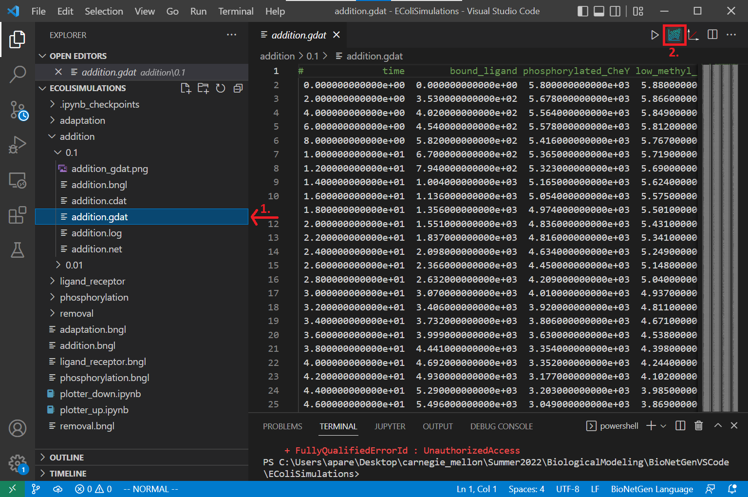
Open the newly created addition.gdat file and create a plot by clicking the Built-in plotting button.

What happens to the concentration of phosphorylated CheY?

Note: You can deselect AllLigand to make the plot of the concentration of phosphorylated CheY easier to see.

Next, try the following few different values for k_add: 0.01, 0.03, 0.05, 0.1, 0.3, 0.5. What do these changing k_add values represent in the simulation? How does the system respond to the different values?

Note: All of your simulation results are stored in the addition/TIME/ directory within your working directory. As you change the value of k_add, rename the directory with the k_add values instead of the timestamp for simplicity.

You will observe that CheY phosphorylation drops gradually first, instead of the instantaneous sharp drop as we add lots of ligand at once. That means, with the ligand concentration increases, the cell is able to continuously lower the tumbling frequency.

Visualizing the results of our simulation

We are now ready to fill in plotter_up.ipynb, a Jupyter notebook that we will use to visualize the outcome of our simulations.

First specify the directories, model name, species of interest, and rates. Put the plotter_up.ipynb file inside the same folder as addition.bngl, or change the model_path below to point at this folder.

#Specify the data to plot here.
model_path = "addition"  #The folder containing the model
model_name = "addition"  #Name of the model
target = "phosphorylated_CheY"    #Target molecule
vals = [0.01, 0.03, 0.05, 0.1, 0.3, 0.5]  #Gradients of interest

We next provide some import statements for needed dependencies.

import numpy as np
import sys
import os
import matplotlib.pyplot as plt
import colorspace

To compare the responses for different gradients, we color-code each gradient. Colorspace is one of the straight-forward ways to set up a color palette. Here we use a qualitative palette with hues (h) equally spaced between [0, 300], and constant chroma (c) and luminance (l) values.

#Define the colors to use
colors = colorspace.qualitative_hcl(h=[0, 300.], c = 60, l = 70, pallete = "dynamic")(len(vals))

The following function loads and parses the data. Once the file containing your data is loaded, we use the first row to investigate which column stores the concentration of the “target” observable species of interest. When we find that target, we will then access the time points and concentrations of this target molecule.

def load_data(val):
    file_path = os.path.join(model_path, str(val), model_name + ".gdat")
    with open(file_path) as f:
        first_line = f.readline() #Read the first line
    cols = first_line.split()[1:] #Get the col names (species names)

    ind = 0
    while cols[ind] != target:
        ind += 1                  #Get col number of target molecule

    data = np.loadtxt(file_path)  #Load the file
    time = data[:, 0]             #Time points
    concentration = data[:, ind]  #Concentrations

    return time, concentration

Now we will write a function to plot the time coordinates on the x-axis and the concentrations of the molecule at these time points on the y-axis. To do so, we will use the Matplotlib plot function to plot concentrations through time for each gradient value. Time-series data will be colored by the color palette we mentioned earlier.

def plot(val, time, concentration, ax, i):
    legend = "k = " + str(val)
    ax.plot(time, concentration, label = legend, color = colors[i])
    ax.legend()

    return

The plotting function above needs to be initialized with a figure defined by the subplot function. We loop through every gradient concentration to perform the plotting. Afterward, we define labels for the x-axis and y-axis, figure title, and tick lines. The call to plt.show() displays the plot.

fig, ax = plt.subplots(1, 1, figsize = (10, 8))
for i in range(len(vals)):
    val = vals[i]
    time, concentration = load_data(val)
    plot(val, time, concentration, ax, i)

plt.xlabel("time (s)")
plt.ylabel("concentration (#molecules)")
plt.title("Phosphorylated CheY vs time")
ax.minorticks_on()
ax.grid(b = True, which = 'minor', axis = 'both', color = 'lightgrey', linewidth = 0.5, linestyle = ':')
ax.grid(b = True, which = 'major', axis = 'both', color = 'grey', linewidth = 0.8 , linestyle = ':')

plt.show()

Now run the notebook. How do changing values of k_add impact the CheY-P concentrations? Why do you think this is?

In the main text, we will examine the results of our plots and discuss how they can be used to infer the cell’s behavior in the presence of increasing attractant.

Return to main text