Solutions

How do E. coli respond to repellents?

Exercise 1

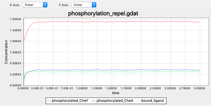
In contrast to that CheY phosphorylations decrease and tumbling becomes less frequent when the cell senses higher attractant concentrations, when the cell senses more repellents there should be more frequent tumbling. The decreased tumbling frequency should be a result of increased CheY phosphorylations. The cell should always be able to adapt to the current concentrations, therefore we also expect the CheY phosphoryaltions be restored when adpating.

Exercise 2

Update reaction rule for ligand-receptor binding from

BoundTP: L(t!1).T(l!1,Phos~U) -> L(t!1).T(l!1,Phos~P) k_T_phos*0.2

BoundTP: L(t!1).T(l!1,Phos~U) -> L(t!1).T(l!1,Phos~P) k_T_phos*5

The complete code (you can download a completed BioNetGen file here: exercise_repel.bngl):

begin model

begin molecule types
	L(t)             #ligand molecule
	T(l,Phos~U~P)    #receptor complex
	CheY(Phos~U~P)
	CheZ()
end molecule types

begin parameters
	NaV2 6.02e8   #Unit conversion to cellular concentration M/L -> #/um^3
	L0 5e3          #number of ligand molecules
	T0 7000       #number of receptor complexes
	CheY0 20000
	CheZ0 6000

	k_lr_bind 8.8e6/NaV2   #ligand-receptor binding
	k_lr_dis 35            #ligand-receptor dissociation
	k_T_phos 15            #receptor complex autophosphorylation
	k_Y_phos 3.8e6/NaV2    #receptor complex phosphorylates Y
	k_Y_dephos 8.6e5/NaV2  #Z dephosphorylates Y
end parameters

begin reaction rules
	LR: L(t) + T(l) <-> L(t!1).T(l!1) k_lr_bind, k_lr_dis

	#Free vs. ligand-bound receptor complexes autophosphorylates at different rates
	FreeTP: T(l,Phos~U) -> T(l,Phos~P) k_T_phos
	BoundTP: L(t!1).T(l!1,Phos~U) -> L(t!1).T(l!1,Phos~P) k_T_phos*5

	YP: T(Phos~P) + CheY(Phos~U) -> T(Phos~U) + CheY(Phos~P) k_Y_phos
	YDeps: CheZ() + CheY(Phos~P) -> CheZ() + CheY(Phos~U) k_Y_dephos
end reaction rules

begin species
	L(t) L0
	T(l,Phos~U) T0*0.8
	T(l,Phos~P) T0*0.2
	CheY(Phos~U) CheY0*0.5
	CheY(Phos~P) CheY0*0.5
	CheZ() CheZ0
end species

begin observables
	Molecules phosphorylated_CheY CheY(Phos~P)
	Molecules phosphorylated_CheA T(Phos~P)
	Molecules bound_ligand L(t!1).T(l!1)
end observables

end model

generate_network({overwrite=>1})
simulate({method=>"ssa", t_end=>3, n_steps=>100})

The simulation outputs:

What if there are multiple attractant sources?

Exercise 1:

In molecule types and observables, update L(t) and T(l,r,Meth~A~B~C,Phos~U~P) to L(t,Lig~A~B) and T(l,r,Lig~A~B,Meth~A~B~C,Phos~U~P), where A and B represent the two ligand types. Update the reaction rule

LR: L(t) + T(l) <-> L(t!1).T(l!1) k_lr_bind, k_lr_dis

L1R: L(t,Lig~A) + T(l,Lig~A) <-> L(t!1,Lig~A).T(l!1,Lig~A) k_lr_bind, k_lr_dis
L2R: L(t,Lig~B) + T(l,Lig~B) <-> L(t!1,Lig~B).T(l!1,Lig~B) k_lr_bind, k_lr_dis

Also update the species by equally split the initial receptor concentrations by 2.

You can download a completed BioNetGen file here: exercise_twoligand.bngl.

Exercise 2:

To wait for adaptation to ligand A, we could replace the forward reaction rate with this rule: rate constant = 0 unless after adapting to A. We could run the simulation without B first and observe the equilibrium methylation states, and use this for deciding whether the cell is adapted to A. (Why not equilibrium concentrations of free A?) One possible implementation is the following: replace

L1R: L(t,Lig~A) + T(l,Lig~A) <-> L(t!1,Lig~A).T(l!1,Lig~A) k_lr_bind, k_lr_dis
L2R: L(t,Lig~B) + T(l,Lig~B) <-> L(t!1,Lig~B).T(l!1,Lig~B) k_lr_bind, k_lr_dis

with

L1R: L(t,Lig~A) + T(l,Lig~A) <-> L(t!1,Lig~A).T(l!1,Lig~A) k_lr_bind, k_lr_dis
L2R: L(t,Lig~B) + T(l,Lig~B) <-> L(t!1,Lig~B).T(l!1,Lig~B) l2rate(), k_lr_dis

and l2rate() is a function defined as (remember to define it before reaction rules)

begin functions
	l2rate() = if(high_methyl_receptor>1.2e3,k_lr_bind,0)
end functions

The complete code:

begin model

begin compartments
  EC  3  100       #um^3
  PM  2  1   EC    #um^2
  CP  3  1   PM    #um^3
end compartments

begin molecule types
	L(t,Lig~A~B)
	T(l,r,Lig~A~B,Meth~A~B~C,Phos~U~P)
	CheY(Phos~U~P)
	CheZ()
	CheB(Phos~U~P)
	CheR(t)
end molecule types

begin observables
	Molecules bound_ligand L(t!1).T(l!1)
	Molecules phosphorylated_CheY CheY(Phos~P)
	Molecules low_methyl_receptor T(Meth~A)
	Molecules medium_methyl_receptor T(Meth~B)
	Molecules high_methyl_receptor T(Meth~C)
	Molecules phosphorylated_CheB CheB(Phos~P)
end observables

begin parameters
	NaV2 6.02e8   #Unit conversion to cellular concentration M/L -> #/um^3
	miu 1e-6

	L0 1e6
	T0 7000
	CheY0 20000
	CheZ0 6000
	CheR0 120
	CheB0 250

	k_lr_bind 8.8e6/NaV2   #ligand-receptor binding
	k_lr_dis 35            #ligand-receptor dissociation

	k_TaUnbound_phos 7.5   #receptor complex autophosphorylation

	k_Y_phos 3.8e6/NaV2    #receptor complex phosphorylates Y
	k_Y_dephos 8.6e5/NaV2  #Z dephosphorylates Y

	k_TR_bind 2e7/NaV2          #Receptor-CheR binding
	k_TR_dis  1            #Receptor-CheR dissociaton
	k_TaR_meth 0.08        #CheR methylates receptor complex

	k_B_phos 1e5/NaV2      #CheB phosphorylation by receptor complex
	k_B_dephos 0.17        #CheB autodephosphorylation

	k_Tb_demeth 5e4/NaV2   #CheB demethylates receptor complex
	k_Tc_demeth 2e4/NaV2   #CheB demethylates receptor complex
end parameters

begin functions
	l2rate() = if(high_methyl_receptor>1.2e3,k_lr_bind,0)
end functions

begin reaction rules
	L1R: L(t,Lig~A) + T(l,Lig~A) <-> L(t!1,Lig~A).T(l!1,Lig~A) k_lr_bind, k_lr_dis
	L2R: L(t,Lig~B) + T(l,Lig~B) <-> L(t!1,Lig~B).T(l!1,Lig~B) l2rate(), k_lr_dis
	#L3R: L(t,Lig~T) + T(l,Lig~O) <-> L(t!1,Lig~O).T(l!1,Lig~O) l2rate(), k_lr_dis

	#Receptor complex (specifically CheA) autophosphorylation
	#Rate dependent on methylation and binding states
	#Also on free vs. bound with ligand
	TaUnboundP: T(l,Meth~A,Phos~U) -> T(l,Meth~A,Phos~P) k_TaUnbound_phos
	TbUnboundP: T(l,Meth~B,Phos~U) -> T(l,Meth~B,Phos~P) k_TaUnbound_phos*1.1
	TcUnboundP: T(l,Meth~C,Phos~U) -> T(l,Meth~C,Phos~P) k_TaUnbound_phos*2.8
	TaLigandP: L(t!1).T(l!1,Meth~A,Phos~U) -> L(t!1).T(l!1,Meth~A,Phos~P) 0
	TbLigandP: L(t!1).T(l!1,Meth~B,Phos~U) -> L(t!1).T(l!1,Meth~B,Phos~P) k_TaUnbound_phos*0.8
	TcLigandP: L(t!1).T(l!1,Meth~C,Phos~U) -> L(t!1).T(l!1,Meth~C,Phos~P) k_TaUnbound_phos*1.6

	#CheY phosphorylation by T and dephosphorylation by CheZ
	YP: T(Phos~P) + CheY(Phos~U) -> T(Phos~U) + CheY(Phos~P) k_Y_phos
	YDep: CheZ() + CheY(Phos~P) -> CheZ() + CheY(Phos~U) k_Y_dephos

	#CheR binds to and methylates receptor complex
	#Rate dependent on methylation states and ligand binding
	TRBind: T(r) + CheR(t) <-> T(r!2).CheR(t!2) k_TR_bind, k_TR_dis
	TaRUnboundMeth: T(r!2,l,Meth~A).CheR(t!2) -> T(r,l,Meth~B) + CheR(t) k_TaR_meth
	TbRUnboundMeth: T(r!2,l,Meth~B).CheR(t!2) -> T(r,l,Meth~C) + CheR(t) k_TaR_meth*0.1
	TaRLigandMeth: T(r!2,l!1,Meth~A).L(t!1).CheR(t!2) -> T(r,l!1,Meth~B).L(t!1) + CheR(t) k_TaR_meth*30
	TbRLigandMeth: T(r!2,l!1,Meth~B).L(t!1).CheR(t!2) -> T(r,l!1,Meth~C).L(t!1) + CheR(t) k_TaR_meth*3

	#CheB is phosphorylated by receptor complex, and autodephosphorylates
	CheBphos: T(Phos~P) + CheB(Phos~U) -> T(Phos~U) + CheB(Phos~P) k_B_phos
	CheBdephos: CheB(Phos~P) -> CheB(Phos~U) k_B_dephos

	#CheB demethylates receptor complex
	#Rate dependent on methyaltion states
	TbDemeth: T(Meth~B) + CheB(Phos~P) -> T(Meth~A) + CheB(Phos~P) k_Tb_demeth
	TcDemeth: T(Meth~C) + CheB(Phos~P) -> T(Meth~B) + CheB(Phos~P) k_Tc_demeth

end reaction rules

begin species
	@EC:L(t,Lig~A) L0
	@EC:L(t,Lig~B) L0
	@PM:T(l,r,Lig~A,Meth~A,Phos~U) T0*0.84*0.9*0.5
	@PM:T(l,r,Lig~A,Meth~B,Phos~U) T0*0.15*0.9*0.5
	@PM:T(l,r,Lig~A,Meth~C,Phos~U) T0*0.01*0.9*0.5
	@PM:T(l,r,Lig~A,Meth~A,Phos~P) T0*0.84*0.1*0.5
	@PM:T(l,r,Lig~A,Meth~B,Phos~P) T0*0.15*0.1*0.5
	@PM:T(l,r,Lig~A,Meth~C,Phos~P) T0*0.01*0.1*0.5
	@PM:T(l,r,Lig~B,Meth~A,Phos~U) T0*0.84*0.9*0.5
	@PM:T(l,r,Lig~B,Meth~B,Phos~U) T0*0.15*0.9*0.5
	@PM:T(l,r,Lig~B,Meth~C,Phos~U) T0*0.01*0.9*0.5
	@PM:T(l,r,Lig~B,Meth~A,Phos~P) T0*0.84*0.1*0.5
	@PM:T(l,r,Lig~B,Meth~B,Phos~P) T0*0.15*0.1*0.5
	@PM:T(l,r,Lig~B,Meth~C,Phos~P) T0*0.01*0.1*0.5
	@CP:CheY(Phos~U) CheY0*0.71
	@CP:CheY(Phos~P) CheY0*0.29
	@CP:CheZ() CheZ0
	@CP:CheB(Phos~U) CheB0*0.62
	@CP:CheB(Phos~P) CheB0*0.38
	@CP:CheR(t) CheR0
end species

end model

generate_network({overwrite=>1})
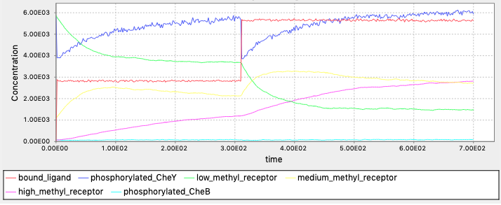
simulate({method=>"ssa", t_end=>700, n_steps=>400})

The simulation outputs:

Exercise 3:

Define ligand_center1 = [1500, 1500] and ligand_center2 = [-1500, 1500]. Since we are considering two gradients, we can add up the ligand concentration. We can replace our cal_concentraion(pos) function with

def calc_concentration(pos):
    dist1 = euclidean_distance(pos, ligand_center1)
    dist2 = euclidean_distance(pos, ligand_center2)

    exponent1 = (1 - dist1 / origin_to_center) * (center_exponent - start_exponent) + start_exponent
    exponent2 = (1 - dist2 / origin_to_center) * (center_exponent - start_exponent) + start_exponent

    return 10 ** exponent1 + 10 ** exponent2

Is the actual tumbling reorientation used by E. coli smarter than our model?

Now, for sampling the new direction, we need to consider the past concentration and the current concentration the bacterium experiences. Since the new direction is also dependent on the last direction, we also need to record the current directions.

Therefore, for our tumble_move() function, we would consider three inputs: curr_direction, curr_conc, past_conc. If the current concentration is higher than the past concentration, we sample the turning with mean of 1.19π-0.1π=1.09π and standard deviation of 0.63π; otherwise ample the turning with mean of 1.19π and standard deviation of 0.63π. The new direction is the sum of the turning and the past direction.

Add the mean and standard deviation of turning as constants.

#Constants for E.coli tumbling
tumble_angle_mu = 1.19
tumble_angle_std = 0.63

We implement the tumble_move function as the following:

def tumble_move(curr_dir, curr_conc, past_conc):
    #Sample the new direction
    corrent = curr_conc > past_conc

    if correct:
        new_dir = np.random.normal(loc = tumble_angle_mu - 0.1, scale = tumble_angle_std)
    else:
        new_dir = np.random.normal(loc = tumble_angle_mu, scale = tumble_angle_std)
    new_dir *= np.random.choice([-1, 1])
    new_dir += curr_dir

    new_dir = new_dir % (2 * math.pi) #keep within [0, 2pi]

    projection_h = math.cos(new_dir) #Horizontal displacement for next run
    projection_v = math.sin(new_dir) #Vertical displacement for next run

    tumble_time = np.random.exponential(tumble_time_mu) #Length of the tumbling

    return new_dir, projection_h, projection_v, tumble_time

Update the simulate function by replacing

projection_h, projection_v, tumble_time = tumble_move()

with

curr_direction, projection_h, projection_v, tumble_time = tumble_move(curr_direction, curr_conc, past_conc)

Can’t get enough BioNetGen?

Exercise 1: You should know the molecules involved (molecule types), reactions and reaction rate constants (reaction rules), the initial conditions (species), the quantities you are interested in observing (observables), your simulation methods and time steps. Compartments and parameters should also be considered if applicable.

Exercise 2: The complete code (you can download a completed BioNetGen file here: exercise_polymerization.bngl):

begin model

begin molecule types
	A(h,t)
end molecule types

begin reaction rules
	Initiation: A(h,t) + A(h,t) <-> A(h,t!1).A(h!1,t) 0.01,0.01
	Polymerizationfree: A(h!+,t) + A(h,t) <-> A(h!+,t!1).A(h!1,t) 0.01,0.01
	Polymerizationfree2: A(h,t) + A(h,t!+) <-> A(h,t!1).A(h!1,t!+) 0.01,0.01
	Polymerizationbound: A(h!+,t) + A(h,t!+) <-> A(h!+,t!1).A(h!1,t!+) 0.01,0.01
end reaction rules

begin species
	A(h,t) 1000
end species

begin observables
	Species A1 A==1
	Species A2 A==2
	Species A3 A==3
	Species A5 A==5
	Species A10 A==10
	Species A20 A==20
	Species ALong A>=30
end observables

end model

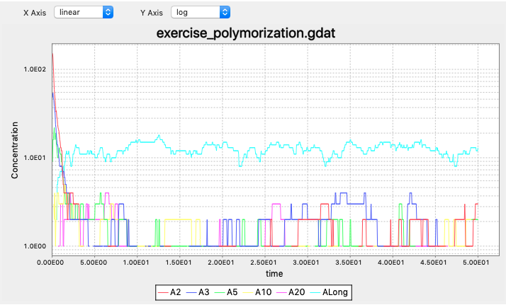
simulate({method=>"nf", t_end=>50, n_steps=>1000})

The simulation outputs (note the concentrations are in log-scale):

How to calculate steady state concentration in a reversible bimolecular reaction?

Exercise 1: When the reaction begins, concentrations change toward the equilibrium concentrations. The system remains at the equilibrium state once reaching it.

Exercise 2: Use [A], [B], [AB] to denote the equilibrium concentrations. At equilibrium concentrations, we have

k_bind · [A] · [B] = k_dissociate · [AB].

Because of conservation of mass, if the instead starts from no AB, our initial conditions will be a₀ = b₀ = 100, and ab₀ = 0. (If we instead work from the “current” concentrations, a₀ = b₀ = 95, and ab₀ = 5, how would you set up the calculations?)

Similar as in the main text, Our original steady state equation can be modified to

k_bind · (a₀ - [AB]) · (b₀ - [AB]) = k_dissociate · [AB].

Solving this equation yields [AB] = 90.488.

Exercise 3: If we add additional 100 A molecules to the system, more AB will be formed. If you use the equation setup in the solution above, we can simply update a₀ = 200. [AB] = 99.019.

If k_dissociate = 9 instead of 3, less AB will be present at the equilibirum state. [AB] = 84.115.

How to simulate a reaction step with the Gillespie algorithm?

Exercise 1: Shorter because molecules collide to each other and react more frequently.

Exercise 2: In this system, we have λ = 100. The probability that exactly 100 reaction happen in the next second is

\[\mathrm{Pr}(X = 100) = \dfrac{\lambda^n e^{-\lambda}}{n!} = 0.03986\,.\]

The expected wait time is 1/λ = 0.01.

The probability that the first reaction occur after 0.02 second is

\[\mathrm{Pr}(T > 0.02) = e^{-\lambda t} = 0.1353\,.\]

Exercise 3: At the beginning of the simulation, only one type of reaction could occur: L + T → LT. The rate of reaction is k_bind[L][T] = 100molecule·s^-1. Therefore we have λ = 100molecule·s^-1, and the expected wait time is thus 1/λ = 0.01s·molecule^-1.

Although the expected wait time before the first reaction is considerably shorter than 0.1s, it is still possible for the first reaction to happen after 0.1s.

After the first reaction, our system has 9 L, 9 T, and 1 LT molecules. There are two possible types of reactions to occur: the forward reaction L + T → LT and the reverse reaction LT → L + T. The rate of forward reaction is k_bind[L][T] = 81molecule·s^-1, while the rate of reverse reaction is k_dissociate[LT] = 2molecule·s^-1. The total reaction rate is 83molecule·s^-1 and hence the expected wait time before the next reaction is 0.012s. The probability of forward reaction is 81molecule·s^-1/83molecule·s^-1 = 0.976, and the probability of reverse reaction is 0.0241.