 Leanpub
In this tutorial, we will use Python to build a Jupyter notebook. We suggest only following the tutorial closely if you are familiar with Python or programming in general. If you have not installed Python, then the following software and packages will need to be installed:
| Installation Link | Version1 | Check Install |
|---|---|---|
| Python3 | 3.7 | python –version |
| Jupyter Notebook | 4.4.0 | jupyter –version |
| matplotlib | 2.2.3 | conda list or pip list |
| numpy | 1.15.1 | conda list or pip list |
| scipy | 1.1.0 | conda list or pip list |
| imageio | 2.4.1 | conda list or pip list |
You can read more about various installation options here or here.
Once you have Jupyter Notebook installed, create a new notebook file called diffusion_automaton.ipynb.
Note: You will need to save this file on the same level as another folder named /dif_images. ImageIO will not always create this folder automatically, so you may need to create it manually.
You may also download the completed tutorial here.
We are now ready to simulate our automaton representing the diffusion of two particle species: a prey (A) and a predator (B). Enter the following into our notebook.
import matplotlib.pyplot as plt
import numpy as np
import time
from scipy import signal
import imageio

%matplotlib inline

images = []
To simulate the diffusion process, we will rely upon an imported convolution function. The convolve function will use a specified 3 x 3 laplacian matrix to simulate diffusion as discussed in the main text. Specifically, the convolve function in this case takes two matrices, mtx and lapl, and uses lapl as a set of multipliers for each square in mtx. We can see this operation in action in the image below.
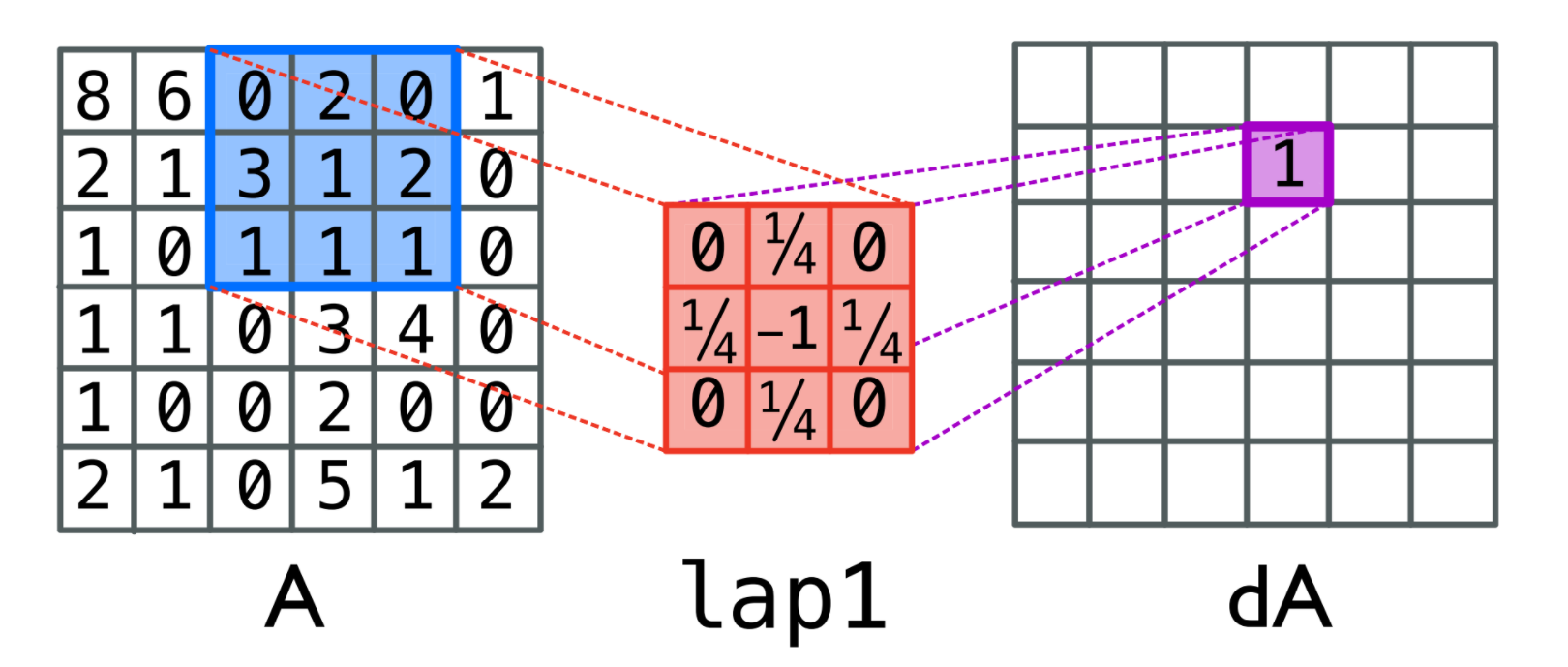 A single step in the convolution function which takes the first matrix and adds up each cell multiplied by the number in the second matrix. Here we see (0 * 0) + (2 * ¼) + (0 * 0) + (3 * ¼) + (1 * -1) + (2 * ¼) + (1 * 0) + (1 * ¼) +(1 * 0) = 1
Because we’re trying to describe the rate of diffusion over this system, the values in the 3 x 3 laplacian excluding the center sum to 1. In our code, the value in the center is -1 because we’ve specified the change in the system with the convolution function i.e. the matrix dA, which we then add to the original matrix A. Thus the total sum of the laplacian is 0 which means the total change in number of molecules due to diffusion is 0, even if the molecules are moving to new locations. We don’t want any new molecules created due to just diffusion! (This would violate the law of conservation of mass.)
We are now ready to write a Python function Diffuse that we will add to our notebook. This function will take a collection of parameters:
numIter: the number of steps to run our simulationA,B: matrices containing the respective concentrations of prey and predators in each celldt: the unit of timedA,dB: diffusion rates for prey and predators, respectivelylapl: our 3 x 3 Laplacian matrixplot_iter: the number of steps to “skip” when animating our simulation
def Diffuse(numIter, A, B, dt, dA, dB, lapl, plot_iter):
    print("Running Simulation")
    start = time.time()

    # Run the simulation
    for iter in range(numIter):
        A_new = A + (dA * signal.convolve2d(A, lapl, mode='same', boundary='fill', fillvalue=0)) * dt
        B_new = B + (dB * signal.convolve2d(B, lapl, mode='same', boundary='fill', fillvalue=0)) * dt
        A = np.copy(A_new)
        B = np.copy(B_new)
        if (iter % plot_iter is 0):
            plt.clf()
            plt.imshow((B / (A+B)),cmap='Spectral')
            plt.axis('off')
            now = time.time()
            # print("Seconds since epoch =", now-start)
            # plt.show()
            filename = 'dif_images/diffusion_'+str(iter)+'.png'
            plt.savefig(filename)
            images.append(imageio.imread(filename))

    return A, B
The following parameters will set up our problem space by defining the grid size, the number of iterations we will range through, and establishing the initial matrices A and B.
# _*_*_*_*_*_*_*_*_* GRID PROPERTIES *_*_*_*_*_*_*_*_*_*
grid_size = 101 # Needs to be odd
numIter = 10000;
seed_size = 11 # Needs to be an odd number
A = np.ones((grid_size,grid_size))
B = np.zeros((grid_size,grid_size))

# Seed the predators
B[int(grid_size/2)-int(seed_size/2):int(grid_size/2)+int(seed_size/2)+1, \
int(grid_size/2)-int(seed_size/2):int(grid_size/2)+int(seed_size/2)+1] = \
np.ones((seed_size,seed_size))
The following parameters will establish the time step, the diffusion rates, and how many steps will be between frames of our animation.
# _*_*_*_*_*_*_*_*_* SIMULATION VARIABLES *_*_*_*_*_*_*_*_*_*
dt = 1.0
dA = 0.5
dB = 0.25
lapl = np.array([[0.05, 0.2, 0.05],[0.2, -1.0, 0.2],[0.05, 0.2, 0.05]])
plot_iter = 50

Diffuse(numIter, A, B, dt, dA, dB, lapl, plot_iter)
imageio.mimsave('dif_images/diffusion_movie.gif', images)
We now are ready to save and run our notebook. When you run the notebook, you should see an animation in which concentrations of predators are spreading out against a field of prey.
As we return to the main text, we will discuss this animation and extend our model to be able to handle reactions as well as diffusion.
-
Other versions may be compatible with this code, but those listed are known to work for this tutorial ↩
