A Coarse-Grained Model of Particle Diffusion

A coarse-grained model of single particle diffusion

Part of a modeler’s job is to find simple models that capture the essence of a system while running quickly and scaling well to larger inputs.

Our model consumes a huge amount of computational resources because it must track the movements of hundreds of thousands of individual particles. Our goal is to build a “coarse-grained” model that will allow us to witness Turing patterns emerge without the computational overhead required to track individual particles.

We will grid off a two-dimensional plane into blocks and store only the concentration of each type of particle found within each block. To simplify things further, we will assume that the concentration of a particle in each block is represented by a decimal number (sometimes representing a percentage concentration) as opposed to counting individual particles.

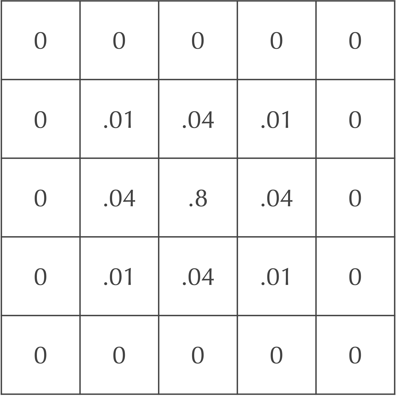
We will begin with an example of the diffusion of only A particles; we will later add B particles as well as reactions to our model. Say that the particles have concentration equal to 1 in the central cell of the grid and 0 everywhere else, as shown below.

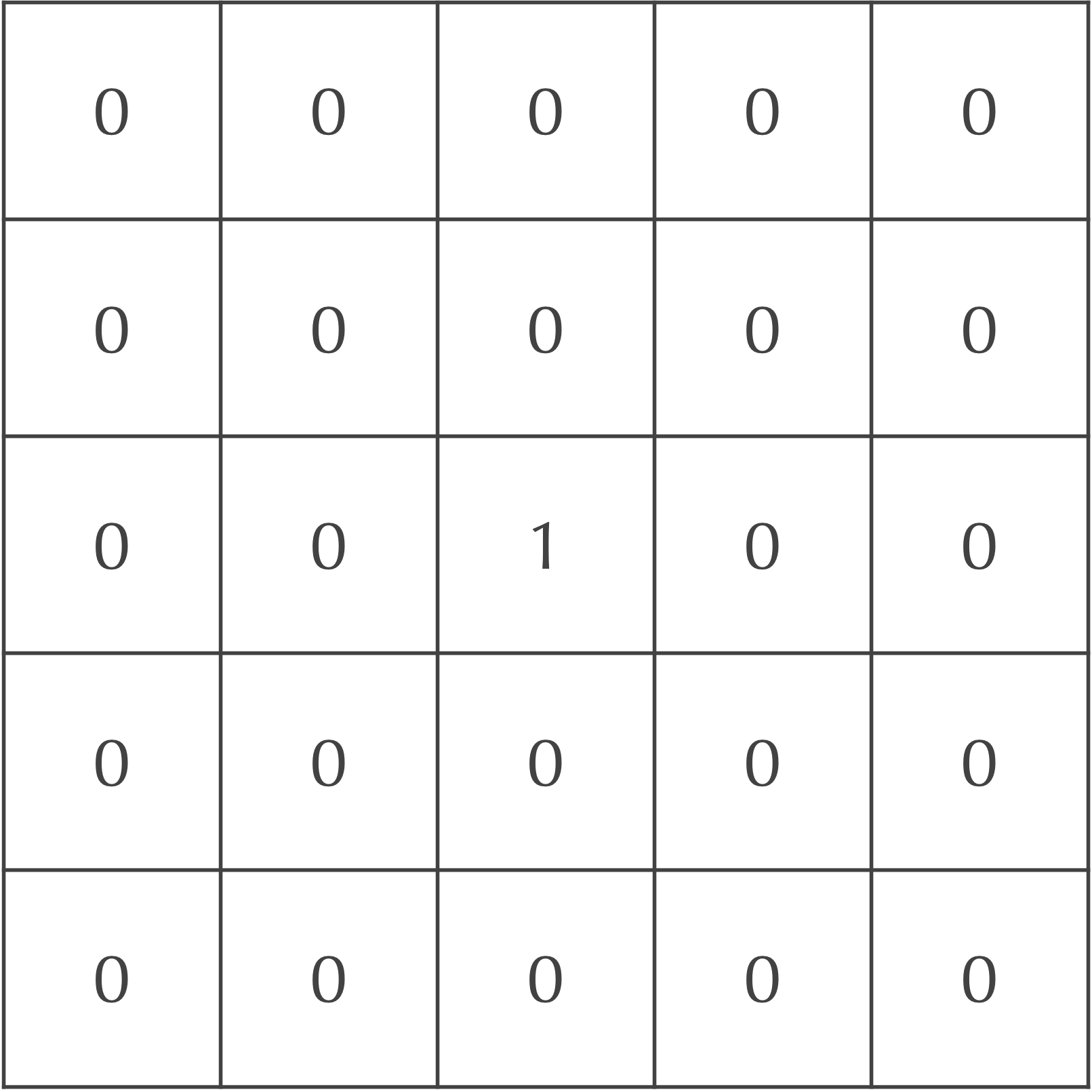A 5 x 5 grid showing hypothetical initial concentrations of A particles. Cells are labeled by decimal numbers representing their concentration of A particles. The central cell has maximum concentration, and no particles are contained in any other cell.

We will now update the grid of cells after one time step to mimic particle diffusion. To do so, we will spread out the concentration of particles in each square to its eight neighbors. For example, we could assume that 20% of the current cell’s concentration diffuses to each of its four adjacent neighbors, and that 5% of the cell’s concentration diffuses to each of its four diagonal neighbors. Because the central square in our ongoing example is the only cell with nonzero concentration, the updated concentrations after a single time step are shown in the following figure.

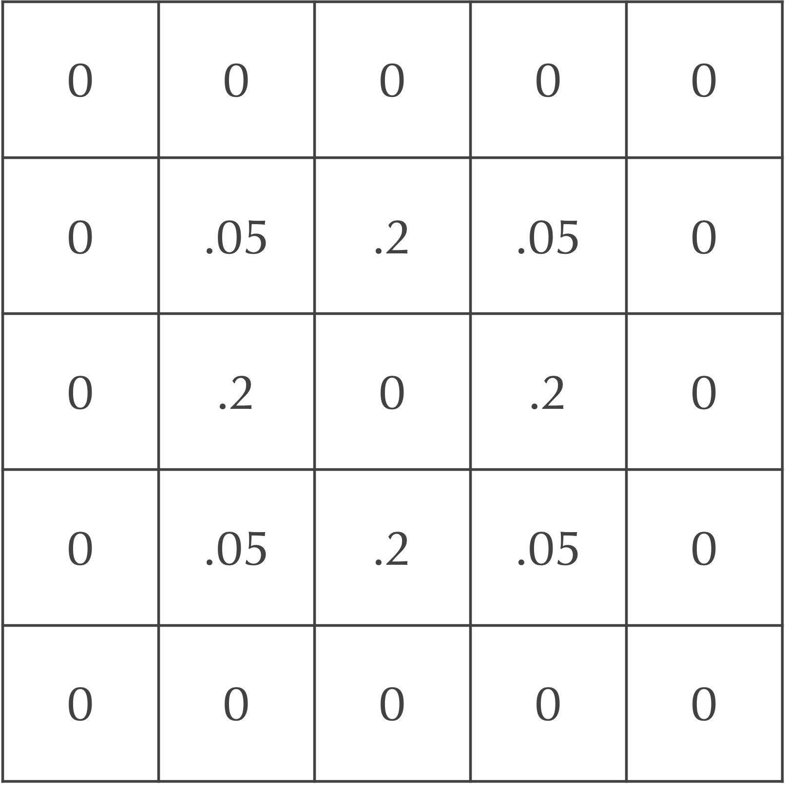A grid showing an update to the system in the previous figure after diffusion of particles after a single time step.

Note: The sum of the values in both grids in the figure above is equal to 1, which ensures the conservation of total mass in the system.

After an additional time step, the particles continue to diffuse outward. For example, each diagonal neighbor of the central cell in the above figure, which has a concentration of 0.05 after one time step, will lose all of its particles in the following step. Each of these cells will also gain 20% of the particles from two of its adjacent neighbors, along with 5% of the particles from the central square (whose concentration is zero). This makes the updated concentration of this cell after two time steps equal to 2(0.2)(0.2) + 0.05(0) = 0.08.

The four cells directly adjacent to the central square, which have a concentration of 0.2 after one time step, will also gain particles from their neighbors. Each such cell will receive 20% of the particles from two of its adjacent neighbors and 5% of the particles from two of its diagonal neighbors, which have a concentration of 0.2. Therefore, the updated concentration of each of these cells after two time steps is 2(0.2)(0.05) + 2(0.05)(0.2) = 0.02 + 0.02 = 0.04.

Finally, the central square has no particles after one step, but it will receive 20% of the particles from each of its four adjacent neighbors, as well as 5% of the particles from each of its four diagonal neighbors. As a result, the central square’s concentration after two time steps is 4(0.2)(0.2) + 4(0.05)(0.05) = 0.17.

In summary, the central nine squares after two time steps are as shown in the following figure.

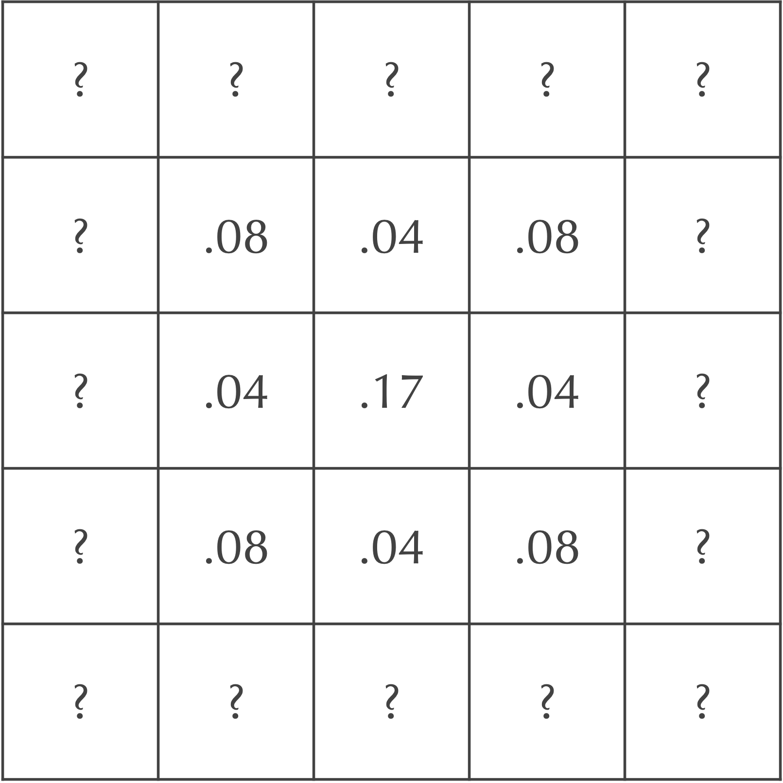A grid showing an update to the central nine squares of the diffusion system in the previous figure after an additional time step. The cells labeled “?” are left as an exercise for the reader.

STOP: What should the values of the “?” cells be in the above figure?

The coarse-grained model of particle diffusion that we have built is a variant of a cellular automaton, or a grid of cells in which we use fixed rules to update the status of a cell based on its current status and those of its neighbors. Cellular automata form a rich area of research applied to a wide variety of fields dating back to the middle of the 20th Century; if you are interested in learning more about them from the perspective of programming, then you might like to check out the Programming for Lovers project.

Slowing down the diffusion rate

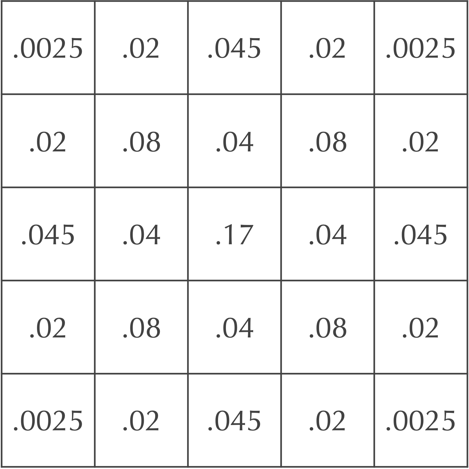
There is just one problem: our diffusion model is too volatile! The figure below shows the initial automaton as well as its updates after each of two time steps. In a true diffusion process, all of the particles would not rush out of the central square in a single time step, only for some of them to return in the next step.

A 5 x 5 cellular automaton model for diffusion of a single particle. (Left) The system contains a maximum concentration of particles in the central square. (Center) The system after one time step. (Right) The system after two time steps.

Our solution is to slow down the diffusion process by adding a parameter d_A having values between 0 and 1 that represents the rate of diffusion of A particles. Instead of moving a cell’s entire concentration of particles to its neighbors in a single time step, we move only a fraction d_A of them.

Revisiting our original example, say that d_A is equal to 0.2. After the first time step, only 20% of the central cell’s particles will be spread to its neighbors. Of these particles, 5% will be spread to each diagonal neighbor, and 20% will be spread to each adjacent neighbor. The figure below illustrates that after one time step, the central square has concentration equal to 0.8, its adjacent neighbors have concentration equal to 0.2d_A = 0.04, and its diagonal neighbors have concentration equal to 0.05d_A = 0.01.

An updated grid of cells showing the concentration of A particles after one time step if d_A = 0.2.

Adding a second particle to our diffusion simulation

We now will add B particles to the simulation, which we assume also start with concentration equal to 1 in the central square and 0 elsewhere. Recall that B, our “predator” molecule, diffuses half as fast as A, the “prey” molecule. If we set the diffusion rate d_B equal to 0.1, then our cells after a time step will be updated as shown in the figure below. This figure represents the concentration of the two particles in each cell as an ordered pair ([A], [B]).

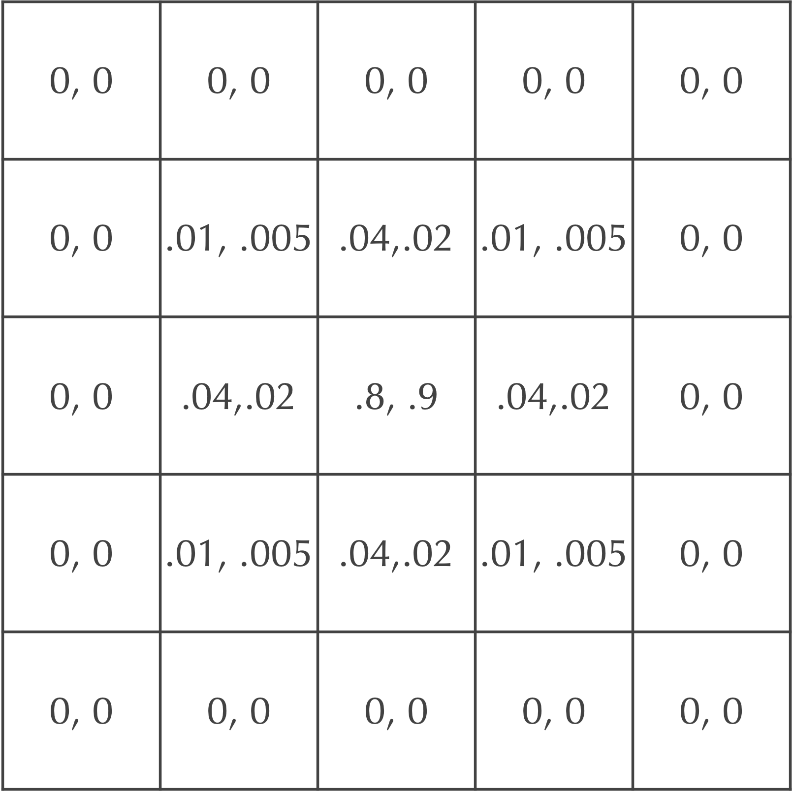A figure showing cellular concentrations after one time step for two particles A and B that start at maximum concentration in the central square and diffuse at rates d_A = 0.2 and d_B = 0.1. Each cell is labeled by the ordered pair ([A], [B]).

STOP: Update the cells in the above figure after another generation of diffusion. Use the diffusion rates d_A = 0.2 and d_B = 0.1.

Visualizing particle concentrations in an automaton

As we move toward diffusing a large board that is hundreds of cells wide, listing the concentrations of our two particles in each cell will be difficult to analyze. Instead, we need some way to visualize the results of our diffusion simulation.

First, we will consolidate the information stored in a cell about the concentrations of two particles into a single value. In particular, let a cell’s particle concentrations be denoted [A] and [B]. Then the single value [B]/([A] + [B]) is the ratio of the concentration of B particles to the total number of particles in the cell. This value ranges between 0 (no B particles present) and 1 (only B particles present).

STOP: What should be the value of [B]/([A] + [B]) if both [A] and [B] are equal to zero?

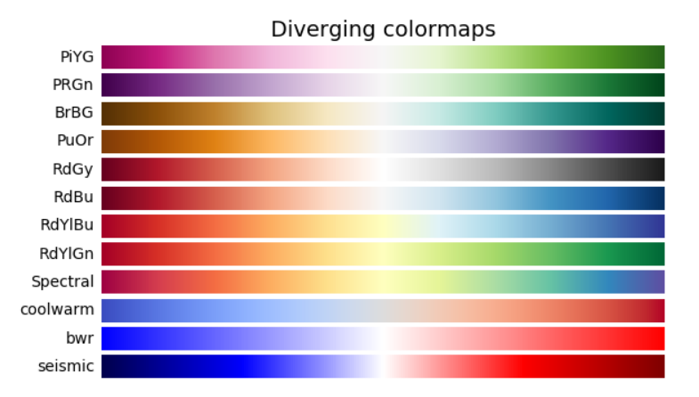
Next, we color each cell according to its value of [B]/([A] + [B]) using a color spectrum like those shown in the figure below. We will use the Spectral color map, meaning that if a cell has a value close to 0 (relatively few predators), then it will be colored red, while if it has a value close to the maximum value of [B]/([A] + [B]) (relatively many predators), then it will be colored dark blue.

When we color each cell over many time steps, we can animate the automaton to see how it changes over time. We are now ready for the following tutorial, in which we will implement and visualize our diffusion automaton using a Jupyter notebook.

Visit tutorial

The video below shows an animation of a 101 x 101 board with d_A = 0.5 and d_B = 0.25 that begins with [A] = 1 for all cells. All cells have [B] = 0 except for an 11 x 11 square in the middle of the grid, where [B] = 1. (There is nothing special about the dimensions of this central square.) Without looking at individual concentration values, this animation allows us to see immediately that the A particles are remaining in the corners, while a band of B particles expands outward from the center.

Note: Particles technically “fall off” the sides of the board in the figure below, meaning that a given particle’s total concentration across all cells decreases over time.

Next lesson