Turing Pattern Exercises

Solar photons and random walks

Photons are massless particles carrying electromagnetic radiation. In the sun’s core, photons are created as the result of nuclear fusion when two hydrogen atoms crash together and form a helium atom. The photons that are released have a great deal of kinetic energy, traveling at the speed of light (approximately 300,000,000 m/s). However, the atoms in the center of the sun are densely packed together, and so just like proteins in the cytoplasm, photons constantly bounce off atoms and follow random walks.

The average distance that a photon travels between atom collisions is called the photon’s “mean free path”. The mean free path varies depending on the photon’s distance from the sun’s core, but conservative estimates of the average mean free path dictate that it is no more than 1 cm.

Exercise: On average, what is the length of each step of a solar photon’s random walk? That is, based on a mean free path of 1 cm, what is the typical time between collisions for a given photon traveling at the speed of light?

When you feel the warmth of sunshine, the photons colliding with your skin have traveled from the sun in just eight minutes. But how long did these photons take to reach the surface of the sun in the first place?

Exercise: Use the Random Walk Theorem to approximate the number of steps that it will take for a photon to reach the sun’s corona from its center, given that the sun has a radius of 700,000 km. Then, use your solution to the previous exercise to estimate the expected time required for this journey.

Practicing the cellular automaton model of diffusion

Earlier in this module, we showed a grid of cells containing concentrations of two particles A and B that start with concentration equal to 1 in the central square and diffuse according to the rates d_A = 0.2 and d_B = 0.1. In a “STOP” question, we asked you to update this grid, reproduced below, after another time step of diffusion.

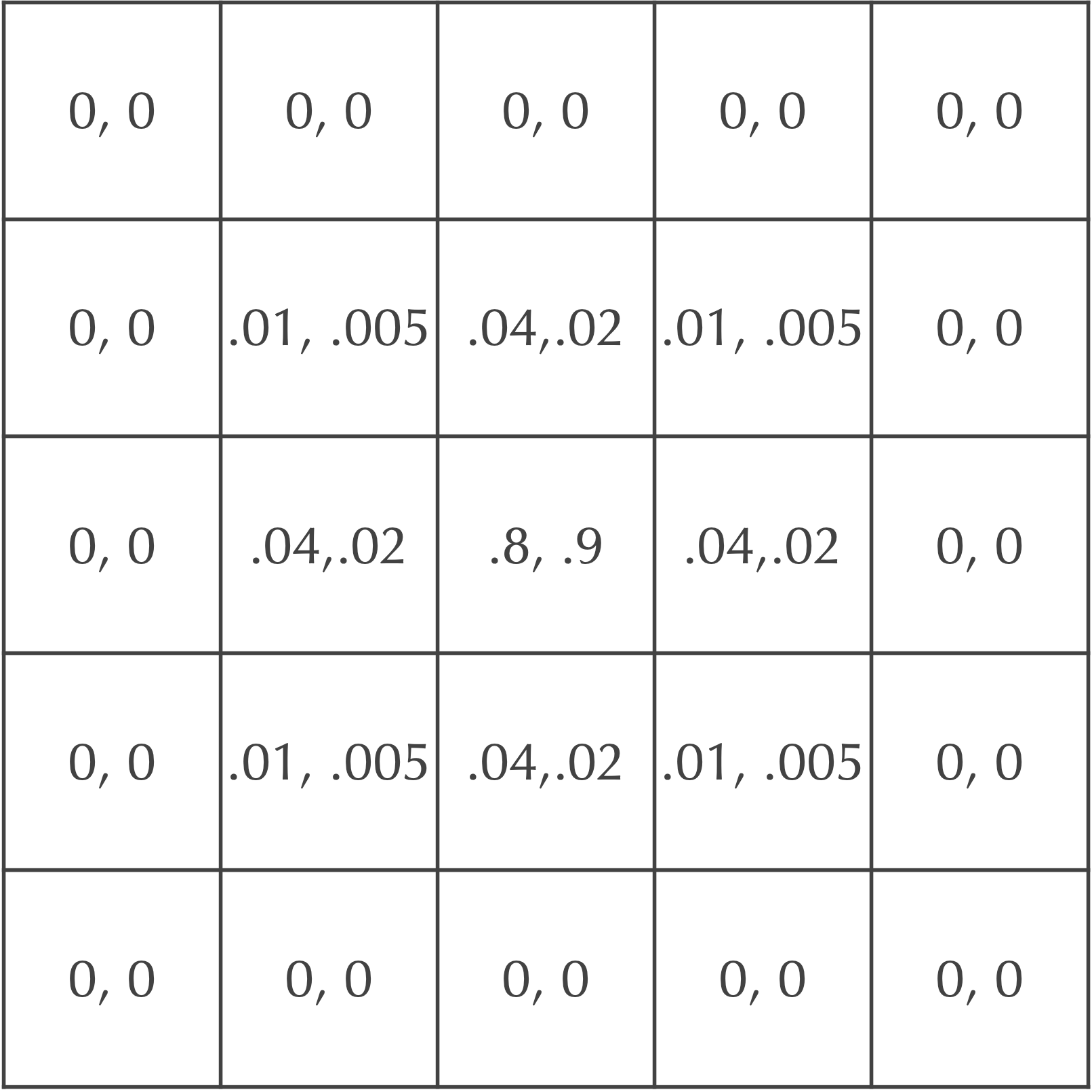A figure showing cellular concentrations after one time step for two particles A and B that start at maximum concentration in the central square and diffuse at rates d_A = 0.2 and d_B = 0.1. Each cell is labeled by the ordered pair ([A], [B]).

Exercise: Instead of solely diffusing the particles, update the original grid (in which A and B have concentration equal to 1 in the central cell) for two time steps according to the Gray-Scott model. Use f = 0.03 and k = 0.1.

Changing the predator-prey reaction

Both our particle simulator and the Gray-Scott model used a reaction A + 2B → 3B to represent a predator-prey dynamics of sorts. But there is no reason a priori why we would have used this reaction; instead, we could have modeled the simpler reaction A + B → 2B, in which a predator molecule collides with a prey molecule, and the prey molecule changes into a predator. Because this reaction only requires the collision of two particles, it would be more frequent than the reaction A + 2B → 3B if all else is equal.

Exercise: Adapt the particle-based simulation that we introduced earlier in a tutorial to replace the reaction A + B → 3B with A + B → 2B. Play around with the system’s reaction rate parameters; are you still able to generate Turing patterns?

Exercise: How would the simulation from the Gray-Scott tutorial need to change to model the reaction A + B → 2B instead of A + B → 3B? Make the appropriate changes to the implementation of the Gray-Scott model; do you still observe Turing patterns?

Changing Gray-Scott parameters

Recall the figure below, which shows how changing feed and kill rates affect Turing patterns.

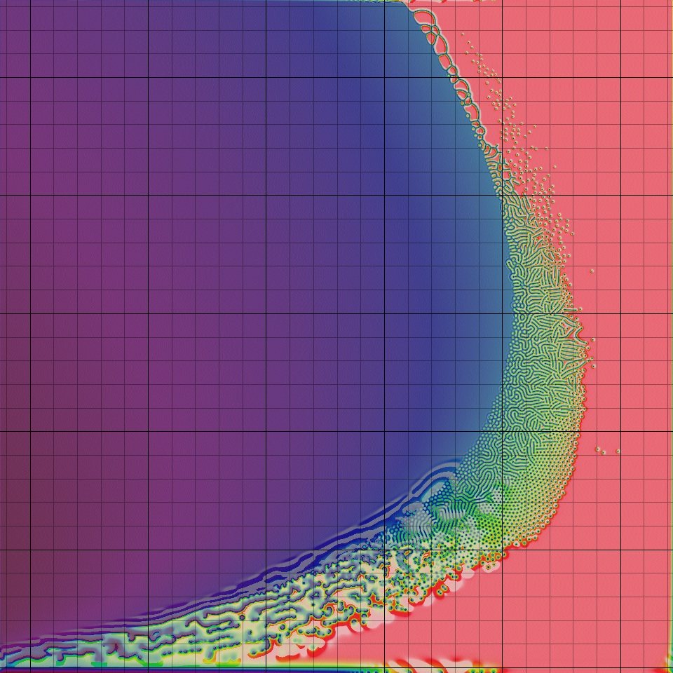Changing kill (x-axis) and feed (y-axis) parameters greatly affects the Turing patterns obtained in the Gray-Scott model. Each small square shows the patterns obtained from a given choice of feed and kill rate. Note that many choices of parameters do not produce Turing patterns, which only result from a narrow “sweet spot” band of parameter choices.

Exercise: Try changing the diffusion rates in the Gray-Scott model to the values of d_{A = 0.1 and dB = 0.05. Do the same patterns result? What happens if we make the diffusion rates equal?}

When we diffuse particles in the automaton model (including the Gray-Scott model), we did not mention what happens at the boundary of the simulation because we were interested in the patterns that arise in the interior of the grid. The simulations shown in the figures in this chapter assume that the automaton is surrounded by a “buffer” of invisible cells that have zero concentration. In this way, the particles leaving the board simply flow off the edges.

We could have used two additional methods to handle barriers. First, we could assume that particles flowing off one side of the board are added to the corresponding cells on the opposite side of the board. Second, we could assume that particles ricochet off the barriers, so that any points that would flow off the side of the board instead remain in the current cell.

In the Gray-Scott tutorial, this was handled by the setting the parameter boundary='fill' to signal.convolve2d(). The boundary parameter could also take the additional options boundary='wrap' or boundary='symm' to represent the above two cases, which can be combined with the \texttt{‘fillvalue’} option as documented here.

Exercise: Adapt the simulation of the Gray-Scott model to handle each of these additional two cases. Do you see the same patterns arise?

Next module