Software Tutorial: Generating Turing Patterns with a Reaction-Diffusion Simulation

Note: We are currently in the process of updating this tutorial to the latest version of MCell, CellBlender, and Blender. This tutorial works with MCell3, CellBlender 3.5.1, and Blender 2.79. Please see the previous tutorial for a link to download these versions.

In this tutorial, we will build the predator-prey reaction-diffusion model that we introduced in the main text. A warning that these simulations can take a long time to run.

Load the CellBlender_Tutorial_Template.blend file that you generated in the Random Walk Tutorial. You may also download the complete file here. Save this file as a new file named turing_pattern.blend. The completed tutorial is also available here.

We will first visit CellBlender > Molecules and create the B molecules, as shown in the screenshot below.

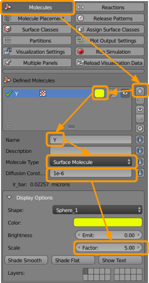
1. Click the + button.
2. Select a color (such as red).
3. Name the molecule B.
4. Under molecule type, select surface molecule.
5. Add a diffusion constant of 3e-6. The diffusion constant indicates how many units to move the particle every time unit. (We will specify the time unit below at runtime.)
6. Up the scale factor to 2 (click and type 2 or use the arrows).

Then, repeat the above steps to make sure that all of the following molecules are entered. We use a molecule named Hidden to represent a “hidden” molecule that will be used to generate A molecules.

Molecule Name	Molecule Type	Color	Diffusion Constant	Scale Factor
B	Surface	Red	3e-6	3
A	Surface	Green	6e-6	3
Hidden	Surface	Blue	1e-6	0

Now visit CellBlender > Molecule Placement to set the following sites for releasing molecules of each of the three types. First, we will release the hidden molecules across the region so that any new A particles will be produced uniformly.

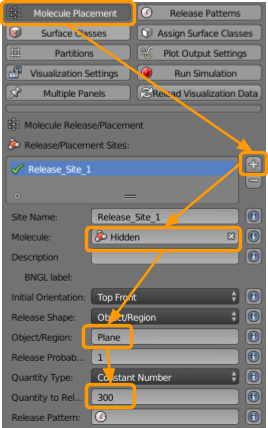
1. Click the + button.
2. Select or type in the molecule Hidden.
3. Type in the name of the Object/Region Plane.
4. Set the Quantity to Release as 1000.

Then, repeat the above steps to release an initial quantity of A molecules as well, using the following table.

Molecule Name	Object/Region	Quantity to Release
Hidden	Plane	1000
A	Plane	6000

We are going to release an initial collection of B particles in a cluster in the center of the plane. To do so, we will need a very specific initial release of these particles, and so we will not be able to use the Molecule Placement tab. For this reason, we need to write a Python script to place these molecules, shown below. You can download this script here. (Don’t worry if you are not comfortable with Python.)

import cellblender as cb
dm = cb.get_data_model()
mcell = dm['mcell']
rels = mcell['release_sites']
rlist = rels['release_site_list']
point_list = []
for x in range(10):
    for y in range(10):
        point_list.append([x/100,y/100,0.0])
for x in range(10):
    for y in range(10):
        point_list.append([x/100 - 0.5,y/100 - 0.5,0.0])
for x in range(10):
    for y in range(10):
        point_list.append([x/100 - 0.8,y/100,0.0])
for x in range(10):
    for y in range(10):
        point_list.append([x/100 + 0.8,y/100 - 0.8,0.0])
new_rel = {
    'data_model_version' : "DM_2015_11_11_1717",
    'location_x' : "0",
    'location_y' : "0",
    'location_z' : "0",
    'molecule' : "B",
    'name' : "pred_rel",
    'object_expr' : "arena",
    'orient' : "'",
    'pattern' : "",
    'points_list' : point_list,
    'quantity' : "400",
    'quantity_type' : "NUMBER_TO_RELEASE",
    'release_probability' : "1",
    'shape' : "LIST",
    'site_diameter' : "0.01",
    'stddev' : "0"
}
rlist.append ( new_rel )
cb.replace_data_model ( dm )

Locate the Outliner pane on the top-right of the Blender screen. On the left of the view button in the Outliner pane, there is a code tree icon.

Click this icon and choose Text Editor. To create a new file for our code, click the + button. Copy and paste the code above (or from your downloaded file) into the text editor and save it with the name pred-center.py.

Next visit CellBlender > Scripting > Data-Model Scripting > Run Script, as shown in the following screenshot. Select Internal from the Data-Model Scripting menu and click the refresh button. Click the filename entry area next to File and enter pred_center.py. Click Run Script to execute.

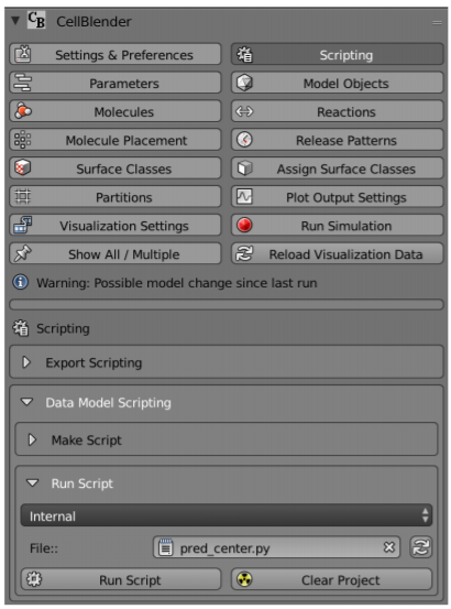
You should see that another placement site called pred_rel has appeared in the Molecule Placement tab.

Next go to CellBlender > Reactions to create the reactions that will drive the system.

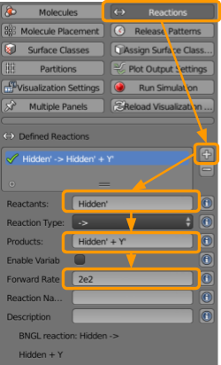
1. Click the + button.
2. Under reactants, type Hidden; (note: the semi-colon is important).
3. Under products, type Hidden; + A;
4. Set the forward rate as 1e5.

Repeat these steps to ensure that we have all of the following reactions.

Reactants	Products	Forward Rate
Hidden;	Hidden; + A;	1e5
B;	NULL	1e5
B; + B; + A;	B; + B; + B;	1e1

We are now ready to run our simulation. To do so, visit CellBlender > Run Simulation and select the following options:

1. Set the number of iterations to 200.
2. Ensure the time step is set as 1e-6.
3. Click Export & Run.

Once the run is complete, save your file.

We can also now visualize our simulation. Click CellBlender > Reload Visualization Data. You have the option of watching the animation within the Blender window by clicking the play button at the bottom of the screen.

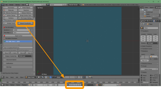
If you like, you can export this animation by using the following steps:

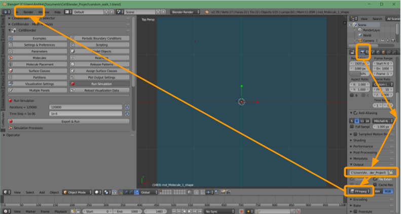
1. Click the movie tab.
2. Scroll down to the file name.
3. Select a suitable location for the file.
4. Select the file type you would like (we suggest FFmpeg_video).
5. Click Render > OpenGL Render Animation.

The movie will begin playing, and when the animation is complete, the movie file should be in the folder location you selected.

You may be wondering how the parameters in the above simulations were chosen. The fact of the matter is that for many choices of these parameters, we will obtain behavior that does not produce an animation as interesting as what we found in this tutorial. Furthermore, try making slight changes to the feed and kill rates in the CellBlender reactions (e.g., multiplying one of them by 1.25) and watching the animation. How does a small change in parameters cause the animation to change?

As we return to the main text, we will discuss how the patterns that we observe change as we make slight changes to these parameters. What biological conclusion can we draw from this phenomenon?

Return to main text