 Leanpub
From random walks to reaction-diffusion
In the previous lesson, we introduced the model of a particle randomly walking through a medium. But what exactly do random walks have to do with Alan Turing and zebras?
Turing’s insight was that remarkable high-level patterns could arise if we combine particle diffusion with chemical reactions, in which colliding particles interact with each other. Such a model is called a reaction-diffusion system, and the emergent patterns are called Turing patterns in his honor.
We will consider a reaction-diffusion system having two types of particles, A and B. The system is not explicitly a predator-prey relationship, but you may like to think of the A particles as prey and the B particles as predators.
Both types of particles diffuse randomly through the plane, but the A particles diffuse more quickly than the B particles. In the simulation that follows, we will assume that A particles diffuse twice as quickly as B particles. In terms of our random walk model, this faster rate of diffusion means that in a single “step”, an A particle moves twice as far as a B particle.
STOP: Say that we release a collection of A and B particles at the same location. If the particles move via random walks, and the A particles diffuse twice as fast as the B particles, then on average, how much farther from the origin will the A particles be than the B particles after n steps?
We now will add three reactions to our system. First, A particles are added into the system at some constant feed rate f. As a result of the feed reaction, the concentration of the A particles increases by a constant number in each time step.
Note: We will work with a two-dimensional simulation, but in a three-dimensional system, the units of f would be in mol/L/s, which means that every second, there are f moles of particles added to the system for every liter of volume. (Recall from your chemistry class long ago that one mole is 6.02214076 · 1023 particles, called Avogadro’s number.)
Second, B particles are removed from the system at a constant kill rate k. As a result of the kill reaction, the number of B particles in the system decreases by a factor of k in a given time step. That is, the more B particles that are present, the more B particles are removed.
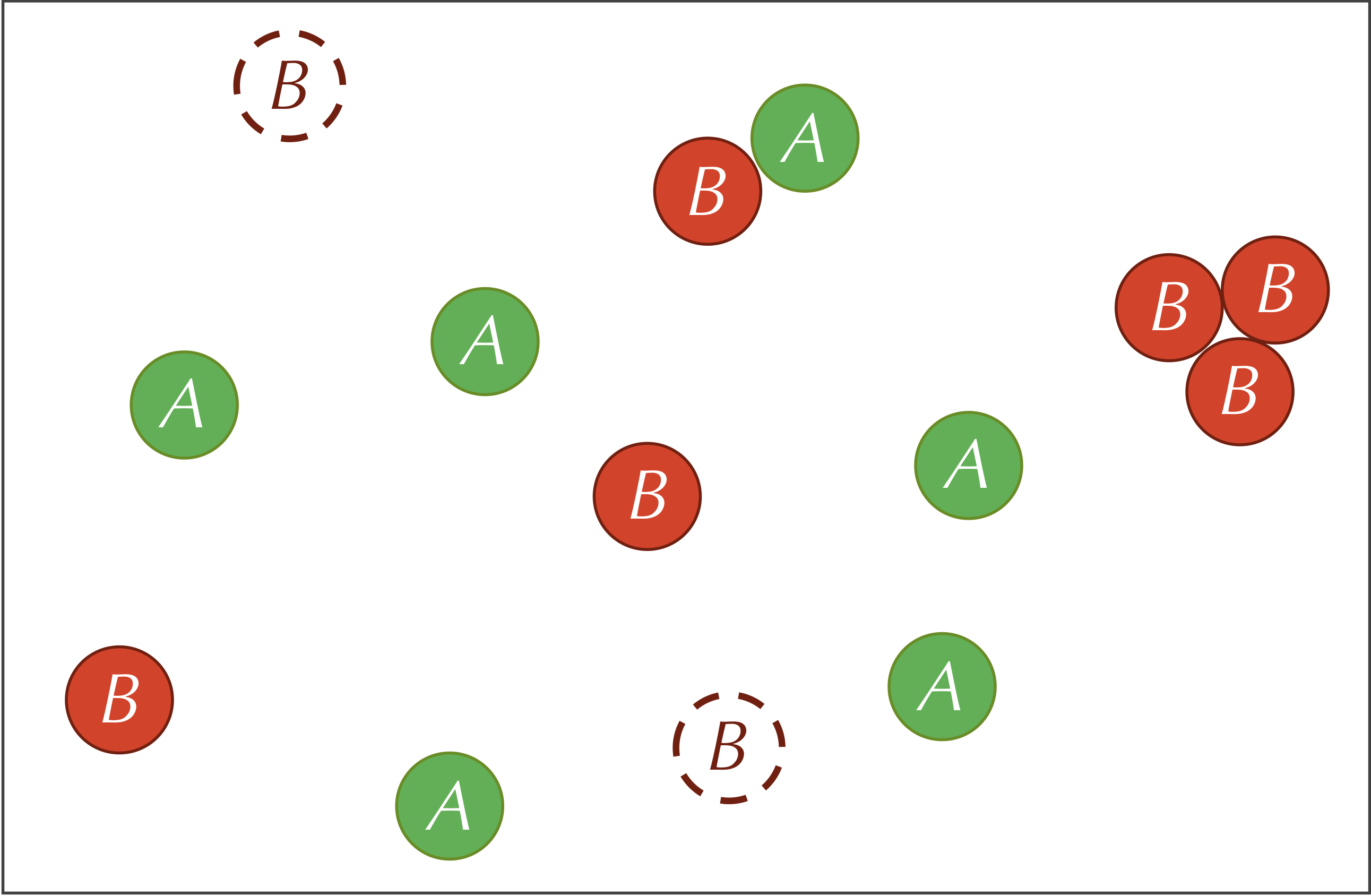
Third, our reaction-diffusion system includes the following reaction involving both particle types. The particles on the left side of this reaction are called reactants and the particles on the right side are called products:
To simulate this reaction on a particle level, if an A particle and two B particles collide with each other, then the A particle has some fixed probability of being replaced by a third B particle, which could vary in practice based on the presence of a catalyst and the orientation of the particles when they collide. This probability directly relates to the rate at which the reaction occurs, denoted r. This third reaction is why we compared A to prey and B to predators, since we may like to conceptualize the reaction as two B particles consuming an A particle and producing a new offspring B particle.
The three reactions defining our system are summarized by the figure below.

Before continuing, we call your attention to a slight difference between the feed and kill reactions. In the feed reaction, the concentration of A particles increases by a constant quantity in each time step. In the kill reaction, the concentration of B particles decreases by a constant factor multiplied by the current concentration of B particles. If we were using calculus to model this system, then letting [A] and [B] denote the concentrations of the two particle types, we would represent the feed and kill reactions by the following two differential equations:
Parameters are omnipresent in biological modeling
A parameter is a variable quantity used as input to a model. Parameters are inevitable in biological modeling (and data science in general), and as we will see, changing parameters can cause major changes in the behavior of a system.
Four parameters are relevant to our reaction-diffusion system: the feed rate (f) of A particles, the kill rate (k) of B particles, the predator-prey reaction rate (r), and the diffusion rate (i.e., speed) of B particles. We do not need to set the diffusion rate of A particles, since we know that their diffusion is twice that of B particles.
We think of all these parameters as dials that we can turn, observing how the system changes as a result. For example, if we raise the diffusion rate, then the particles will be moving around and colliding with each other more, which means that we will see more of the reaction A + 2B → 3B.
STOP: What will happen as we increase or decrease f or k?
In the following tutorial, we will initiate our reaction-diffusion system with a uniform concentration of A particles spread across a two-dimensional plane and a tightly packed collection of B particles in the center of the plane. When we return from this tutorial, we will see if any high-level patterns form.
Changing reaction-diffusion parameters produces different emergent Turing patterns
For many parameter values, our reaction-diffusion system is not very interesting. The following animation is produced when using parameter rates in CellBlender of f = 1000 and k = 500,000. It shows that if the kill rate is too high, then B particles (colored red) will die out more quickly than they can be replenished by the reaction with A particles (colored green), and so only A particles will remain.
Conversely, if f is too high, then the increased feed rate will cause an increase in the concentration of A particles. However, the increased concentration of A particles will also lead to more collisions between A particles and pairs of B particles, causing the concentration of B particles to explode. The following simulation has the parameters f = 1,000,000 and k = 100,000.
The interesting behavior in this system lies in a sweet spot of f and k parameter values. For example, consider the following visualization when f is equal to 100,000 and k is equal to 200,000. We see a clear stripe of B particles expanding outward against a background of A particles, with subsequent stripes appearing at locations where a critical mass of B particles can interact with each other.
When we hold k fixed and increase f to 140,000, the higher feed rate increases the likelihood of B particles encountering A particles, and so we see even more stripes of B particles.
As f approaches k, the stripe structure becomes chaotic and breaks down because many clusters of B particles are now colliding and mixing. The following animation shows the result of raising f to 175,000.
Once f is equal to k, the stripes disappear, as shown in the video below. We might expect this to mean that the A and B particles will be uniformly mixed. Instead, we see that after an initial outward explosion of B particles, the system displays a mottled background. Pay attention to the following video at a point late in the animation. Although the concentrations of the particles are still changing, there is much less large-scale change than in earlier videos. If we freeze the video, our eye cannot help but see patterns of red and green clusters that resemble mottling.
The Turing patterns that emerged from our particle simulations are a testament to the human eye’s ability to find organization within the net behavior of tens of thousands of particles. For example, take another look at the video we produced that showed mottling in our particle simulator. Patterns in this simulation are noisy — even in the dark red regions we will have quite a few green particles, and vice-versa. The rapid inference of large-scale patterns from small-scale visual phenomena is one of the tasks that our brains have evolved to perform well.
You may still be skeptical, since the patterns in the above videos do not have the concrete boundaries that we might expect of animal stripes and spots. Yet when we examine the skin an animal exhibiting Turing patterns, we see the effect of a pointillist painting: the patterns that we infer on a higher level are just the net result of many varied individual points. The figure below shows an example of this effect for zebrafish skin.
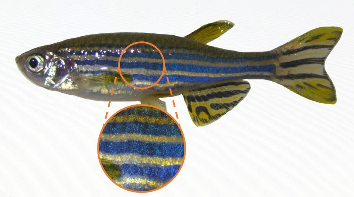 Zooming in on the striped skin of a zebrafish shows that each stripe is formed of many differently colored cells, and that the boundaries of the stripes are more variable than they may seem at lower resolution. Image courtesy: JenniferOwen, Wikimedia Commons (adapted by Kit Yates).
Turing’s patterns and Klüver’s form constants
The particle simulations in the previous subsection may evoke the adjective “trippy”. This is no accident.
Research dating to the 1920s has studied the patterns that humans see during visual hallucinations, which Heinrich Klüver named form constants after studying patients who had taken mescaline.1 These patterns, such as cobwebs, tunnels, and spirals, occur across many individuals, regardless of the cause of their hallucinations.
 A few of Heinrich Klüver’s form constants. Image courtesy: Lisa Diez, Wikimedia Commons.
Over five decades after Klüver’s work, researchers would determine that form constants originate from simpler linear stripes of cellular activation patterns in the retina. When the brain passes these linear patterns from the circular retina to the rectangular field of view interpreted by the visual cortex, it contorts these stripes into form constants.2 Some researchers3 believe that the patterns in the retina caused by hallucinations are in fact Turing patterns and can be explained by a reaction-diffusion model in which one type of neuron acts as a predator and another acts as prey, but this hypothesis remains unresolved.
Streamlining our simulations
Despite using advanced modeling software that has undergone years of development and optimization, each of the simulations in this lesson took several hours to render because they require us to track the movement of tens of thousands of particles over thousands of generations.
We wonder if it is possible to build a model of Turing patterns that does not require so much computational overhead. In other words, is there a simplifying speed-up that we can make to our reaction-diffusion model that will still produce Turing patterns? We will turn our attention to this question in the next lesson.
-
H. Klüver. Mescal and Mechanisms of Hallucinations. University of Chicago Press, 1966. ↩
-
G.B. Ermentrout and J.D. Cowan. “A Mathematical Theory of Visual Hallucination Patterns”. Biol. Cybernetics 34, 137-150 (1979). ↩
-
J. Ouellette. “A Math Theory for Why People Hallucinate”. Quanta Magazine, July 30, 2018. https://www.quantamagazine.org/a-math-theory-for-why-people-hallucinate-20180730/ ↩
